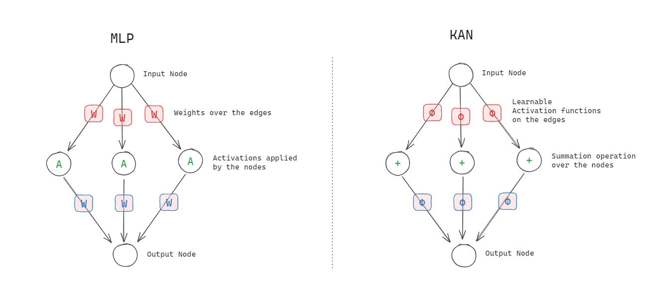
Kolmogorov-Arnold Networks (KANs) Might Change AI As We Know It, Forever
A deep dive into how Kolmogorov-Arnold Networks work, how they differ from Multi-Layer Perceptrons, and how to train one from scratch
A recent pre-print of research published in ArXiv might supercharge the neural networks that we know about today.
These researchers introduced Kolmogorov-Arnold Networks (KANs) which are promising alternatives to the currently dominant Multi-Layer Perceptrons (MLPs) architecture.
This story is a deep dive into what KANs are, how they work, why they might be a great alternative to Multi-Layer Perceptron (MLPs) in the near future, and how to train one from scratch.
But First, What Even Are MLPs?
MLPs or Multi-Layer Perceptrons are fully connected feed-forward neural networks that are at the core of all AI technology that we see today.
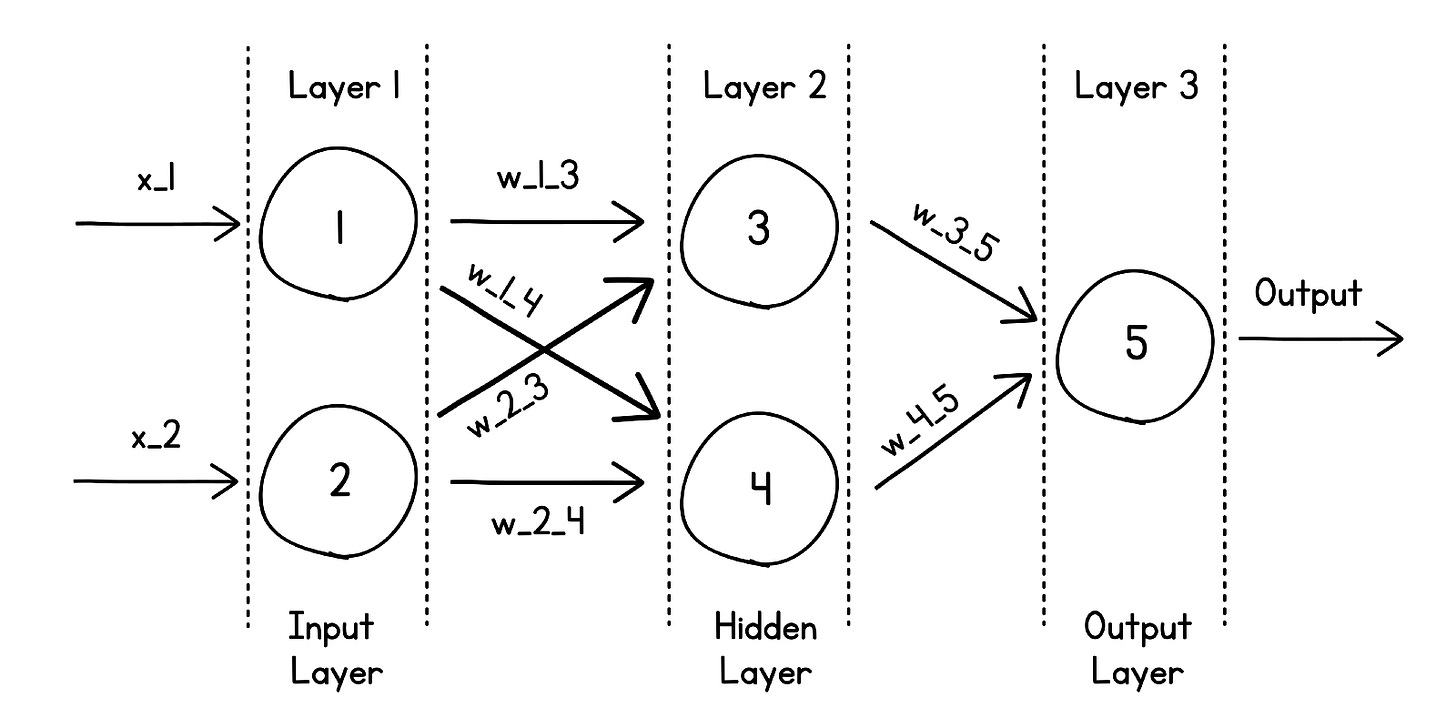
These networks consist of at least three layers of nodes/neurons, namely —
Input layer
Hidden layer(s)
Output layer
Each layer is fully connected to the next or in other words, each node/ neuron in one layer is connected to every node/neuron in the next layer.
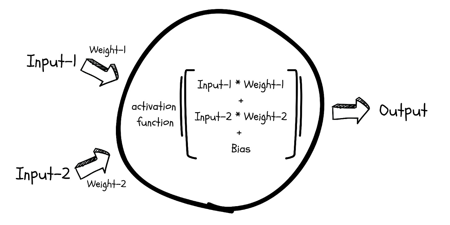
A Node or a Neuron in an MLP uses an Activation function to capture the non-linearities in its input.
These activation functions are fixed and non-linear.
MLPs are inspired by the Universal Approximation Theorem.
This theorem, in easy words, tells that an MLP can approximate any real continuous function to any desired accuracy if it has enough neurons in its hidden layer.
This approximation of an MLP (N(x)) can be mathematically described as follows —
where:
mis the number of neurons in the hidden layerα(i) are the weights on the edges that connecti-th neuron in the hidden layer to the output layerσis the activation functionw(i)are the weights on the edges that connect the input layer to thei-th neuron of the hidden layerxis the input vector to the neural networkb(i)are the biases associated with eachi-th neuron in the hidden layer
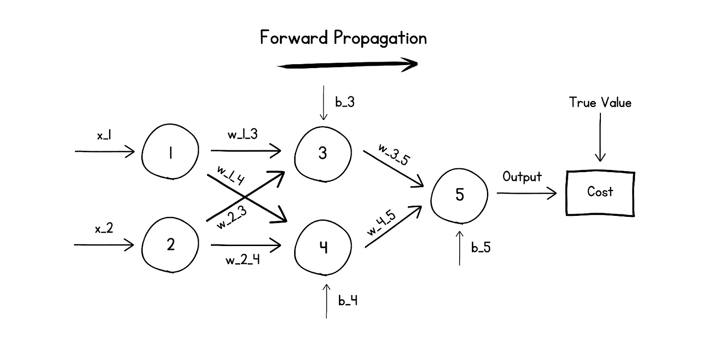
MLPs are predominantly trained using the Gradient Descent-based Backpropagation algorithm that updates its weights and biases based on a Cost function calculated during the Forward Propagation step in the MLP training process.
Now, Coming to KANs and How They Work
KANs are neural networks inspired by the Kolmogorov-Arnold representation theorem (given by the Russian mathematicians, Vladimir Arnold and Andrey Kolmogorov).
This theorem states that every multivariate continuous function can be represented by the summation of continuous univariable functions.
In simple words, it tells that every complex multi-variable function can be broken down into simpler 1-dimensional functions.
The theorem is mathematically described as follows —

where:
f(x)is a multivariate continuous functionx(n)are the input variables of this functionϕ(q,p)andΦ(q)are univariate functions that transform each input variable
In this equation, 2n + 1 signifies the minimum number of univariable functions needed to represent the multivariate continuous function with n inputs.
The function seems to convert any high-dimensional function into its 1-D representations, which can then be learned using conventional machine learning, but this isn’t always true.
The 1-D representations can often be non-smooth (lack a continuous derivative) or can be fractal (infinitely complex and non-differentiable).
Thus, they cannot be learned by gradient-based machine-learning algorithms.
This issue led the Kolmogorov-Arnold representation theorem to a dead end in machine learning in the past.
However, these researchers worked on these limitations by expanding the theorem instead of just relying on a small number (2n+1) of terms in its original representation.
They also noticed that most real-world functions do not lead to non-smooth or fractal representations and thus can be easily learned based on the theorem.
These realisations led to the novel neural network KAN architecture, as described below.
The KAN Neural Network Architecture
In its simplest form, a KAN is similar to the Kolmogorov-Arnold representation theorem equation and consists of just two layers.
The first layer transforms each input using a set of univariate functions.
The second layer summates these transformations and outputs the final prediction.
But when expanded to learn complex real-world functions, KANs consist of multiple layers just like MLPs, where each layer’s output is the input to the next layer.
Multi-layer KANs consist of —
Input layer
Edges (where most computation is performed)
Nodes
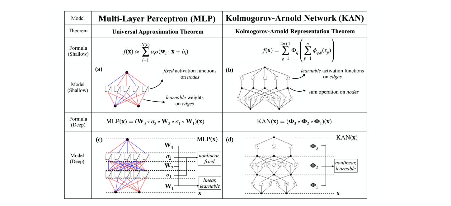
Unlike MLPs where each edge has an associated weight parameter, in a KAN, these weights are completely replaced by learnable univariable functions.
These univariate functions are parameterised using B-Spline.
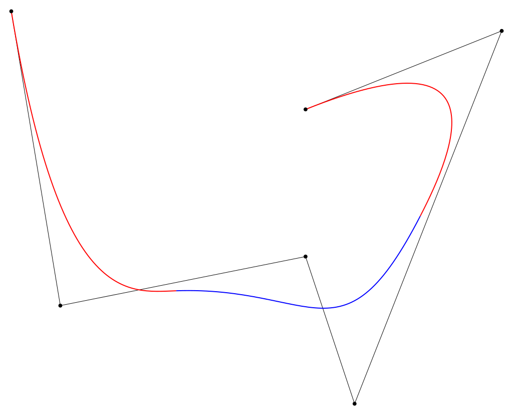
For those new to Splines, these are mathematical functions that let us join a set of points using a smooth curve.
B-Splines or Basis Splines consist of points called Control points that help flexibly manipulate local segments of this smooth curve, without affecting the overall curve.
Coming back, these univariate functions can be thought of as learnable Activation functions present at the edges (rather than in Nodes/ Neurons) of the neural network.
The Nodes in a KAN simply perform the summation of incoming signals instead of applying any Activation function.
Since all operations happening within a KAN are differentiable, they can be trained using Backpropagation with conventional loss functions.
KANs vs. MLPs
The following table in short summarises the differences between KANs and MLPs.
Performance Of KANs
Researchers found that KANs lead to much smaller computational graphs when compared with MLPs.
A 2-layer width-10 KAN is 100 times more parameter efficient (10² vs 10² parameters) than a 4-layer width-100 MLP.
It is also 100 times more accurate than the given MLP (10-⁷ vs 10-⁵ Mean Squared Error).
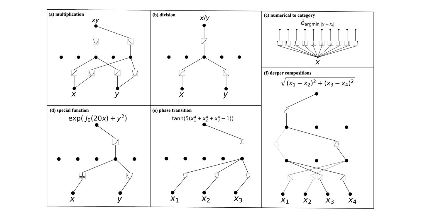
KANs are more effective and accurate at learning and representing various functions as compared to a MLP as shown in the image below.

This accuracy is achieved using fewer parameters than an MLP. In other words, KANs possess faster neural scaling laws than MLPs.
KANs converge faster, achieve lower losses, and have steeper scaling laws than MLPs when used for solving partial differential equations (PDE).

KANs can also be intuitively visualized and can easily interact with humans making them highly interpretable.
By replacing the weight matrices with learnable univariable functions, they can be individually examined to understand how the input features are being transformed at each step in the training process.
This is true for simple symbolic formulae as well as complex mathematical and physical formulae.
When Should You Use KANs?
The researchers provide a useful decision tree that can help us decide when to use KANs vs. MLPs.
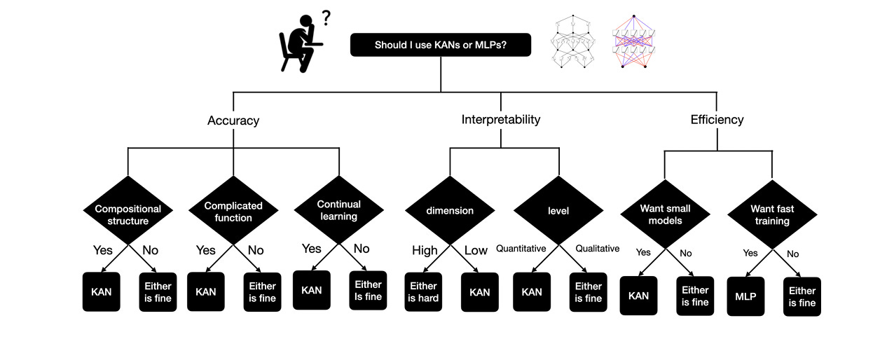
It is to be noted that given the same number of parameters, KANs currently are 10 times slower to train than MLPs.
Thus, in short, if interpretability and accuracy are one’s major requirements and they can compromise on training time, KANs are a great choice for an ML problem.
Learning To Use KANs For Solving ML Problems
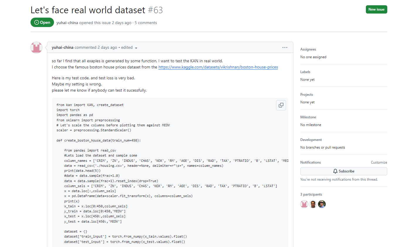
I found an open GitHub issue on the official repository for the project that was about using KANs on the popular Boston house prices dataset.
And, this is the reply from the owner of the project (who is also the first author of the discussed ArXiv pre-print).
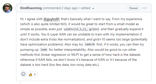
It seems like KANs are quite early for their implementation with many big datasets but we still can use them for many small ML problems.
I would recommend the pykan library documentation as a great resource to learn to build your first KAN.
Here’s an example from it where we build a KAN to solve a binary classification problem over a dataset consisting of points belonging to two interleaving half circles (popularly called two moons).
We first create this dataset using the sklearn library.
from kan import KAN
import matplotlib.pyplot as plt
from sklearn.datasets import make_moons
import torch
import numpy as np

dataset = {}
train_input, train_label = make_moons(n_samples=10000, shuffle=True, noise=0.1, random_state=None)
test_input, test_label = make_moons(n_samples=10000, shuffle=True, noise=0.1, random_state=None)

dataset['train_input'] = torch.from_numpy(train_input)
dataset['test_input'] = torch.from_numpy(test_input)
dataset['train_label'] = torch.from_numpy(train_label)
dataset['test_label'] = torch.from_numpy(test_label)

X = dataset['train_input']
y = dataset['train_label']
plt.scatter(X[:,0], X[:,1], c=y[:])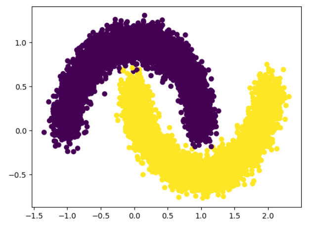
Next, we construct a KAN and train it.
model = KAN(width=[2,2], grid=3, k=3) #KAN with two input and 2 output neurons

def train_accuracy():
    return torch.mean((torch.argmax(model(dataset['train_input']), dim=1) == dataset['train_label']).float())

def test_accuracy():
    return torch.mean((torch.argmax(model(dataset['test_input']), dim=1) == dataset['test_label']).float())

results = model.train(dataset, opt="LBFGS", steps=20, metrics=(train_accuracy, test_accuracy), loss_fn=torch.nn.CrossEntropyLoss())
After this, a symbolic formula is derived that represents what the model has learned from the data.
formula1, formula2 = model.symbolic_formula()[0]

print(formula1)
#1012.55*sqrt(0.6*x_2 + 1) + 149.83*sin(2.94*x_1 - 1.54) - 1075.87

print(formula2)
#-948.72*sqrt(0.63*x_2 + 1) + 157.28*sin(2.98*x_1 + 1.59) + 1010.69
Finally, the accuracy of the learned formula is obtained as follows.
def acc(formula1, formula2, X, y):
    batch = X.shape[0]
    correct = 0
    for i in range(batch):
        logit1 = np.array(formula1.subs('x_1', X[i,0]).subs('x_2', X[i,1])).astype(np.float64)
        logit2 = np.array(formula2.subs('x_1', X[i,0]).subs('x_2', X[i,1])).astype(np.float64)
        correct += (logit2 > logit1) == y[i]
    return correct/batch

print('Training accuracy of the formula:', acc(formula1, formula2, dataset['train_input'], dataset['train_label']))
#Training accuracy of the formula: tensor(1.)

print('Testing accuracy of the formula:', acc(formula1, formula2, dataset['test_input'], dataset['test_label']))
#Testing accuracy of the formula: tensor(0.9990)
And yes, the model performs really well with a testing accuracy of 99.9% when used for this binary classification problem!
Further Reading
Pre-print of the research paper titled ‘KAN: Kolmogorov-Arnold Networks’ on ArXiv
Documentation of ‘pykan’ — the Python implementation of the project
Official GitHub repository of the Kolmogorov Arnold Networks project
What are your thoughts on KANs? Let me know in the comments below.
Also, Restack this story and share it with others, if you found it helpful!


