
A Detailed Guide To Reinforcement Learning From Human Feedback (RLHF) From Scratch
A deep dive into training an LLM and using Reinforcement Learning from Human Feedback (RLHF) with Proximal Policy Optimization (PPO) to align it with human values.


GPT-based LLMs are next-token predictors, and they do their job pretty well.
However, these models have unintended behaviours after Pre-training (training the model for the first time on a huge amount of data).
The first issue is that they do not follow human instructions well.
This can be seen in the following example, where a pre-trained model simply reiterates the instructions in its response.
human_instruction:
"What is the capital of India?"

response_from_pretrained_gpt:
"What is the capital of India? What is capital"
This can be fixed by fine-tuning the model to follow instructions.
Here is how the response from a GPT model might change after fine-tuning it.
human_instruction:
"What is the capital of India?"

response_from_instruction_finetuned_gpt:
"New Delhi"
But the problems do not end here.
The model can make up facts —
response_from_instruction_finetuned_gpt:
"Mumbai"
The model can generate biased or toxic text —
response_from_instruction_finetuned_gpt:
"Isn't it obviously New Delhi?"
Or, the model might choose not to reply at all.
This behaviour is because LLMs are trained with the objective of predicting the next token accurately based on the probability distribution that it had learned from large datasets based on Internet data.
This objective is far from one of following the user’s instructions to respond helpfully and safely.
Or one can say that LLMs are misaligned to this objective.
In 2022, researchers at OpenAI published a useful technique to fix this and ‘align’ GPTs to produce helpful, honest, and harmless responses.
This is called Reinforcement learning from human feedback (RLHF).
OpenAI and Google DeepMind researchers previously used a similar technique for robot locomotion and to play Atari games, achieving remarkable results.

When they used this technique to preference-tune GPT-3 to follow a broad class of written instructions, the resulting model, InstructGPT, was found to be very good at its objective.
In human evaluations, outputs from this 1.3-billion-parameter InstructGPT model were preferred to outputs from the 175-billion-parameter pre-trained GPT-3.
Note that this is the case even though InstructGPT has 100 times fewer parameters!
InstructGPT models also showed improvements in truthfulness and did not produce toxic output as much as compared to the pre-trained GPT-3.
Here is a story where we deep dive into RLHF and learn to implement it from scratch.
Excited? Let’s begin.
But First, How Is GPT-3 Pre-Trained?
GPT-3, or Generative Pre-trained Transformer, is an LLM based on the Transformer architecture.
However, unlike the original Transformer, GPT-3 uses only the Decoder of the Transformer architecture.
This Decoder consists of:
Masked Multi-Head Self-Attention Layers that allow the model to capture dependencies between all tokens in the input sequence.
Feedforward Layers that bring non-linear transformations to the token embeddings.
Layer Normalization that stabilizes training and improves convergence.
Positional Encodings that add sequence order information to tokens.
GPT-3 has a similar architecture as GPT-2, and it has different variants ranging from 125 million parameters to 175 billion parameters (the largest version popularly called “GPT-3”).

GPT-3 was trained on a wide range of datasets that enable it to understand the rules of language.
These datasets include:
Common Crawl: Dataset that represents a large snapshot of the web, filtered to remove irrelevant content
WebText2: Dataset extracted from Reddit links with high karma points
Books1 & Books2: Dataset consisting of collections of books
Wikipedia: Dataset consisting of all English-language Wikipedia articles
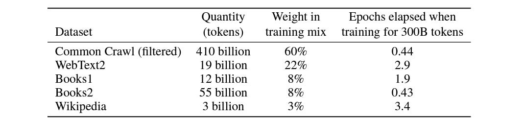
These datasets are combined and pre-processed, and their text is tokenized into subwords using Byte-pair encoding (BPE).
These tokens are converted to Embeddings and are fed to the GPT-3 model, which is trained with Unsupervised learning to predict the next token in the sequence based on the previous tokens.
The loss function minimized during its training is the Negative Log-Likelihood Loss (NLL).
For a sequence of tokens X = { x(1), x(2), … x(N) }, the loss is calculated by taking the negative logarithm of the predicted probability for the correct class.

Given the input token embeddings, the GPT-3 model outputs logits for these.
The softmax function converts these logits into a probability distribution over the vocabulary.
From this distribution, tokens are selected either deterministically (choosing the highest probability token) or probabilistically based on the ‘Temperature’ hyperparameter (for a more creative response).
The selected token IDs are mapped back to their corresponding words or subwords using the tokenizer.
This results in a human-readable output from the GPT model.
Why Is The Pre-trained GPT-3 So Good?
Unlike previous GPT models, the pre-trained GPT-3 model can adapt to different tasks based on user-defined prompts in natural language without requiring any further retraining or fine-tuning.
It can be used for performing different downstream tasks through:
Few-Shot Learning: By giving it a few task-specific examples in the prompt.
# Input:

Classify these as Spam or Not Spam:
1. "You have won a free iPhone! Click here to claim your prize." -> Spam
2. "Your bank account statement is now available online." -> Not Spam
3. "Congratulations, you've been selected for a special offer!" -> Spam
4. "Reminder: Your meeting is scheduled for tomorrow at 3 PM." ->

#Output:

"Not Spam"
One-Shot Learning: By giving it a single task-specific example in the prompt.
# Input:

Translate the following English sentence to German:
Example: "The weather is sunny." -> "Das Wetter ist sonnig."

Next, translate this sentence:
"Where is the nearest train station?" ->

# Output:
"Wo ist der nächste Bahnhof?"
Zero-Shot Learning: By giving it no task-specific examples in the prompt.
# Input:
"What is the capital of India?"

# Output:
"The capital of India is New Delhi"
Next To Supervised Fine-Tuning (SFT)
A team of trained human labellers write up prompts. These, along with prompts sourced from the OpenAI API playground, are combined to produce a prompt dataset.
The labellers then create the desired responses to the prompts in this dataset.
These prompt-response pairs are used to fine-tune the pre-trained GPT-3 with supervised learning.
This process again uses Negative Log-Likelihood Loss (NLL), which measures the difference between the model’s predicted token probabilities and the ground-truth tokens created by labellers.

Training A Reward Model
Starting from the supervised fine-tuned model, its final unembedding layer is removed, and a linear layer that outputs a scalar value representing the reward for each response is added.
This results in a Reward model (RM).
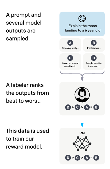
This model takes a prompt and a pair of responses as input and outputs a scalar reward for each response based on how well it aligns with labellers’ preferences (a proxy for human preferences).
The dataset for training the Reward model is derived from human labeller’s comparisons of multiple model outputs for a given prompt.
A 6 billion parameter GPT-3 is supervised fine-tuned and converted into a Reward model, as the larger 175 billion parameter model was found to be unstable when used for this purpose.
The loss function used to train the Reward model is a pairwise ranking loss based on Cross-entropy.

This might look scary, but it is easy to understand.
In the above equation:
xis the given prompty(w)is the preferred completion of the given prompt (as determined by human labellers)y(l)is the less preferred completion for the same promptr(θ)(x,y)is the scalar reward output by the reward model for the promptxand completiony, with parametersθDis the dataset of human-labeled comparisonsKis the number of responses/ completions for a prompt(K 2)or “K choose 2” is the number of unique pairwise comparisons that can be made betweenKresponses.
The sigmoid function (σ) in the above equation converts the reward difference into a probability.
The term E represents the expected value/ average over the dataset D of human-labeled comparisons.
The term 1/(K 2) normalizes the loss over all possible pairwise response comparisons for a prompt in the dataset.
Without this, the prompts with more responses (K) would dominate the loss function, resulting in imbalanced training.
The negative sign of the loss indicates that the Reward model training is a minimization problem.
Overall, the loss function penalizes the Reward model if it assigns a higher reward to the less preferred response.
Finally, To Reinforcement Learning
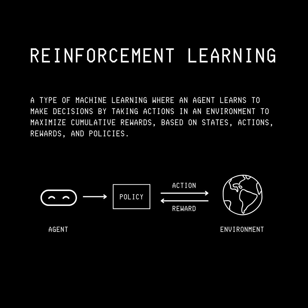
Reinforcement learning (RL), a subset of machine learning, is next used to preference-tune the supervised fine-tuned GPT.
A typical Reinforcement learning setting consists of:
Agent: The decision maker/ action taker
Environment: The surroundings that give feedback based on the agent’s actions
State: The representation of the current situation of the Environment
Actions: The set of all possible moves an agent can make in a given state.
Reward: A scalar feedback received by the agent after taking an Action in a particular State
Episode: The complete sequence of interactions between the agent and the environment. It starts from an initial state and ends when a terminal state is reached.
Policy: The agent's strategy to choose actions in a given state. Technically, it is the mapping from a State to a probability distribution over Actions.
Value Functions: Functions that estimate the expected Return or total future rewards from a given State (State-Value function) or State-Action pair (Action-Value function or Q-function) if the agent acts according to a particular policy thereafter.
Advantage Function: A function that quantifies how much better it is to take a specific action at a particular state compared to the average action at that state.
Mathematically, it is the difference between the Q-function (Action-Value function) and the State-Value function.
With RL, an agent’s objective is to find a policy that maximizes the expected cumulative reward (or Return) over time.
The future rewards are commonly discounted using Discount Factor, a term that reduces the weight of future rewards.
This is based on the idea that immediate rewards are more valuable than the distant ones.
We will revisit more RL fundamentals soon. Let’s return to the original topic for now.
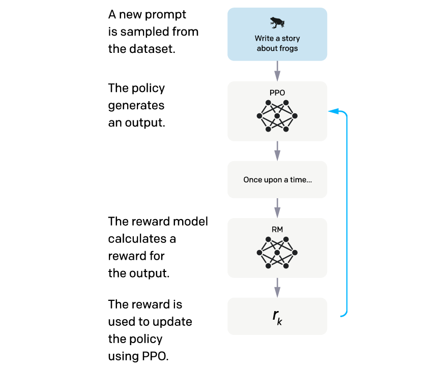
The process of preference tuning GPT starts with setting up a single-arm bandit environment.
This means an agent can interact with a single action or ‘arm’ in this environment.
The agent in this setting is the supervised fine-tuned GPT model.
The action space of the agent consists of all possible token sequences it can generate.
Since the model can generate outputs (Actions) based on the given prompt (State), its internal state (or simply itself) is considered the baseline Policy and termed π(SFT) .
The goal of the agent is to optimize its policy to produce responses that are aligned with human values. This learned policy after RL training is termed π(ϕ)(RL) where ϕ are its parameters.
Time for training!
An episode starts with the environment presenting a single random prompt x (State) to the agent and expecting a response y from it (Action).
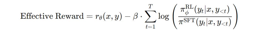
The agent’s response is evaluated by the previously trained Reward Model (part of the environment) and a reward (r(θ)(x,y)) is returned by it as feedback.
This one-step process marks the end of an Episode.
During preference training via RL, the agent can find and exploit patterns in the Reward Model (due to biases in its training) that make it return high rewards for the agent responses.
Such responses could still be undesirable when humans evaluate them.
To ensure this doesn’t happen, a penalty is applied to each token the agent produces.
This penalty is based on the Kullback-Leibler (KL) divergence between the responses generated by the policy in training (π(ϕ)(RL)) and the baseline policy (π(SFT)).
This might all seem very complicated, but it’s really simple to understand.
Kullback–Leibler (KL) divergence simply measures how two probability distributions differ.
The KL divergence in our case is shown in the following equation —
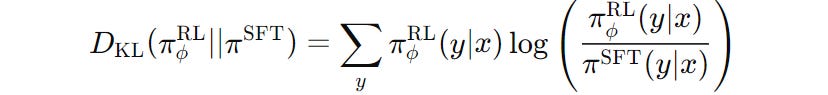
π(ϕ)(RL) (y∣x), and by the baseline SFT GPT model/ policy π(SFT)(y∣x)This value is calculated for both models/policies at each token generation step rather than being calculated over the entire output sequence at once.
For a single output token y(t) at time step t, the per-token KL divergence is proportional to the term below —

This term acts as a penalty to the reward generated by the Reward model and makes sure that the trained policy/ model doesn’t deviate too far from the baseline SFT policy/ model.
Coming back, the RL preference tuning objective that we aim to maximize can be expressed as —
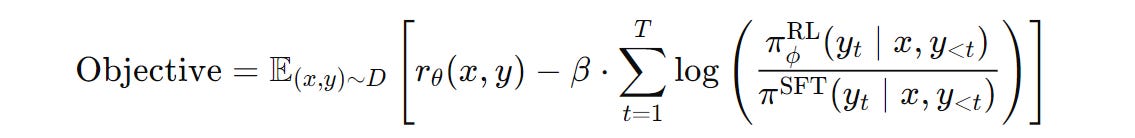
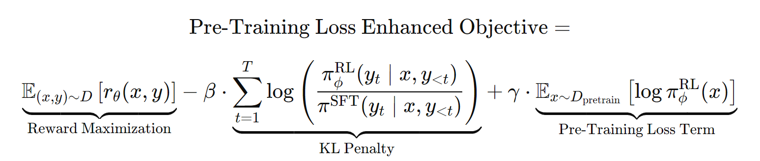
It is seen that Preference-tuning can lead to the model's poor performance on general natural language processing (NLP) tasks, which the pre-trained model was good at.
Thus, a pre-training loss term is added to the above objective.
This acts as a form of regularization and balances the model’s alignment with the reward model while still preserving the knowledge from the original pre-trained language model.
This term is the log-likelihood of sequences from the pre-training data (D(pretrain)) under the trained RL model/policy π(ϕ)(RL).

Adding this term (with a hyperparameter γ that controls its strength) to the previous objective results in the following equation —
Next, we use an RL algorithm called Proximal Policy Optimization (PPO) to maximize this objective.
A Detour Into Proximal Policy Optimization (PPO)
Time for some more RL fundamentals.
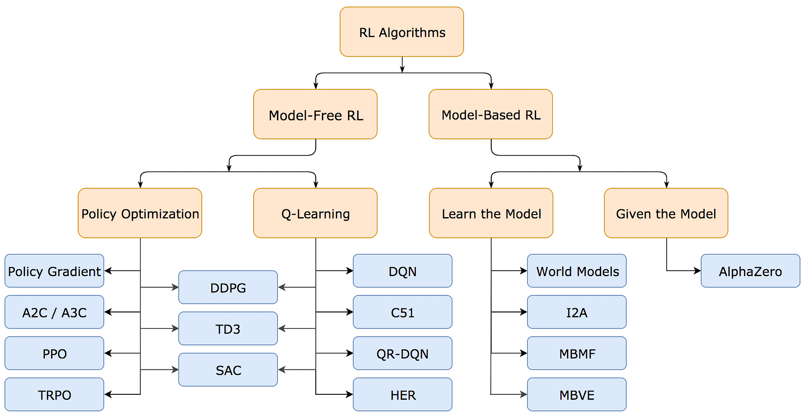
Earlier, we learned that an Agent's goal is to optimize its policy and gain the maximum rewards from its environment.
For this, an agent might or might not have access to (or learn) the model of its environment (i.e. the function which predicts state transitions and rewards).
If it does, the agent can think ahead and decide between actions to take at a given state.
Such an approach is called Model-based reinforcement learning.
A popular example is AlphaZero, an RL model that achieves superhuman performance in Chess, Shogi, and Go.
Commonly, the exact model of the environment is not available to the agent and learning it from the agent’s experience is extremely difficult.
This leads to another approach, called Model-free reinforcement learning, which is easier to implement.
Models in this category can either:
Learn Value functions (commonly the Q-function or the Action-Value function) and are called Value-Based Methods
Learn the policy directly without relying on Value functions, and are called Policy-Based Methods
The one that we’re interested in are the Policy-based methods.
These methods can work with continuous action spaces and where the agent’s policies are stochastic.
The key idea behind these methods is to optimize an agent's policy by finding policy parameters that result in the maximum expected cumulative reward.
The foundation for policy gradient methods is the Policy Gradient Theorem.

Q (π) (s,a) is the Q-function that represents the expected cumulative reward when an action 'a’ is taken at state 's’ and policy π is followed thereafter.This equation describes how to change the policy parameters to increase the expected return.
Mathematically, it describes the gradients of the expected return J(θ) with respect to the policy parameters θ.
By computing them, we can perform Gradient Ascent or update the parameters in the direction that increases the expected return.
Many algorithms developed over the Policy Gradient Theorem but were difficult to work with.
The reason for this was:
Unstable learning due to the high variance of gradients
Requirement for a large number of samples from the environment
Sensitivity and difficulty in finding the correct Learning rate (LR) during training
An algorithm published by OpenAI researchers in 2015 called Trust Region Policy Optimization (TRPO) addressed these challenges.
The idea behind TRPO is to limit the policy change at each update to ensure stable and guaranteed monotonic improvement.
TRPO’s objective uses the Kullback-Leibler (KL) divergence to achieve this by ensuring that the updated policy doesn’t deviate much from the previous one.
Unfortunately, TRPO is tough to implement and uses second-order derivatives, which makes it slow and computationally expensive.
To fix this, another algorithm called Proximal Policy Optimization (PPO) was published by OpenAI in 2017.
PPO is far simpler to implement, can achieve effective learning with fewer samples, and has similar stability to TRPO.
How Does PPO Optimize The Preference Tuning Objective?
Remember the preference tuning objective that we previously defined?
PPO is used to maximize this objective in a stable and efficient way by modifying the parameters of the RL policy ϕ.
To ensure that there are no drastic policy updates, a ratio between the old and updated policy is first calculated.
PPO then uses a Clipped surrogate objective (shown below) that:
Clips this policy ratio to stay within the bounds of
1 − ϵto1 + ϵ(whereϵis a small constant)Multiplies both the clipped and unclipped ratios by the Advantage function
Takes the minimum of these two terms to update the policy

where:
A(t)is the Advantage function, which tells how much better an action is (as per its received reward) than the expected value of the current state.r(t)(ϕ)is the ratio of the updated and the old policy probabilitiesϵis a small constant that limits how muchr(t)(ϕ)changes, ensuring that the updates are not too large
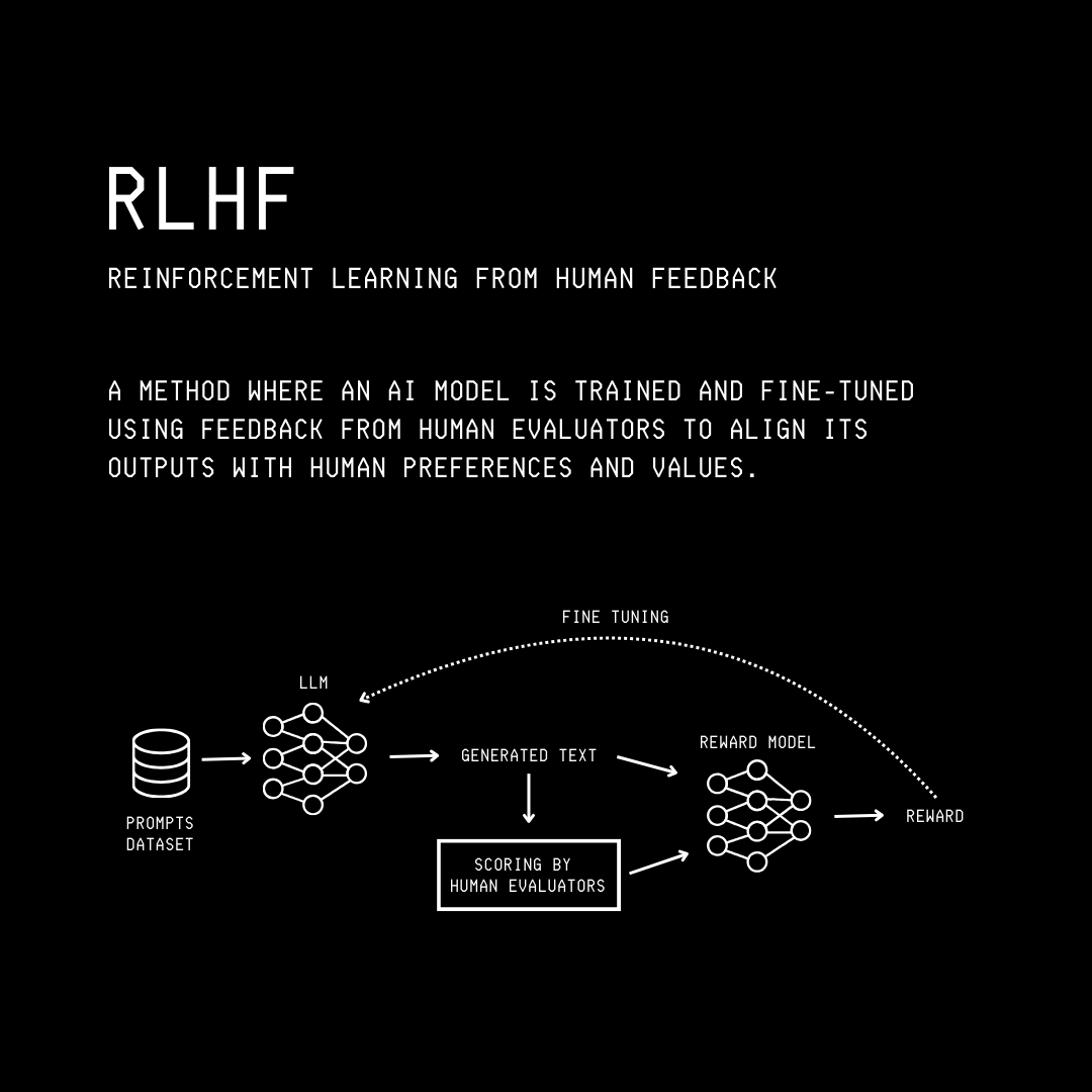
What Is Reinforcement Learning From Human Feedback (RLHF) Finally?
The complete process described above can be summarised in three steps:
Supervised fine-tuning (SFT) of a pre-trained GPT model
Reward model training
Preference tuning of supervised fine-tuned GPT using the Reward model with Reinforcement learning via Proximal Policy Optimization (PPO)
This is called Reinforcement Learning From Human Feedback (RLHF).
How Well Does This Technique Work?
In the original research paper, the GPT tuned by the RLHF process described above is termed InstructGPT.
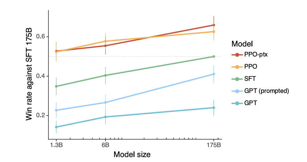
Results show that InstructGPT significantly outperforms the other baselines, with the outputs from the 1.3 billion parameter preference-tuned GPT preferred to those from the 175 billion parameter supervised fine-tuned GPT-3.
Note that in the plots below:
‘PPO-ptx’ is the GPT preference tuned with the objective with the pre-training loss included
‘PPO’ is the GPT preference tuned with the objective where the pre-training loss is not included
‘SFT’ is the supervised fine-tuned GPT model
‘GPT’ is the baseline pre-trained model
‘GPT (prompted)’ is the pre-trained model prompted in a few-shot fashion to follow instructions
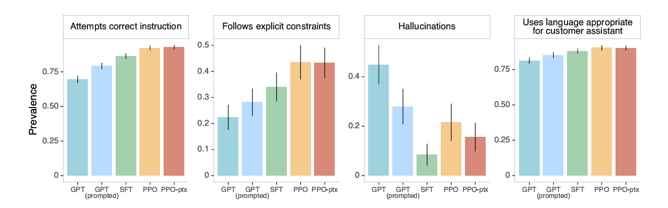
The preference-tuned GPT is better at correctly responding to and in the context of the customer request, follows the mentioned constraints, and is less likely to hallucinate.
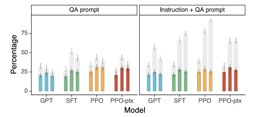
When given question-answering tasks (with and without additional prompts to avoid giving false answers), preference-tuned GPT is slightly more truthful and informative than the baselines.
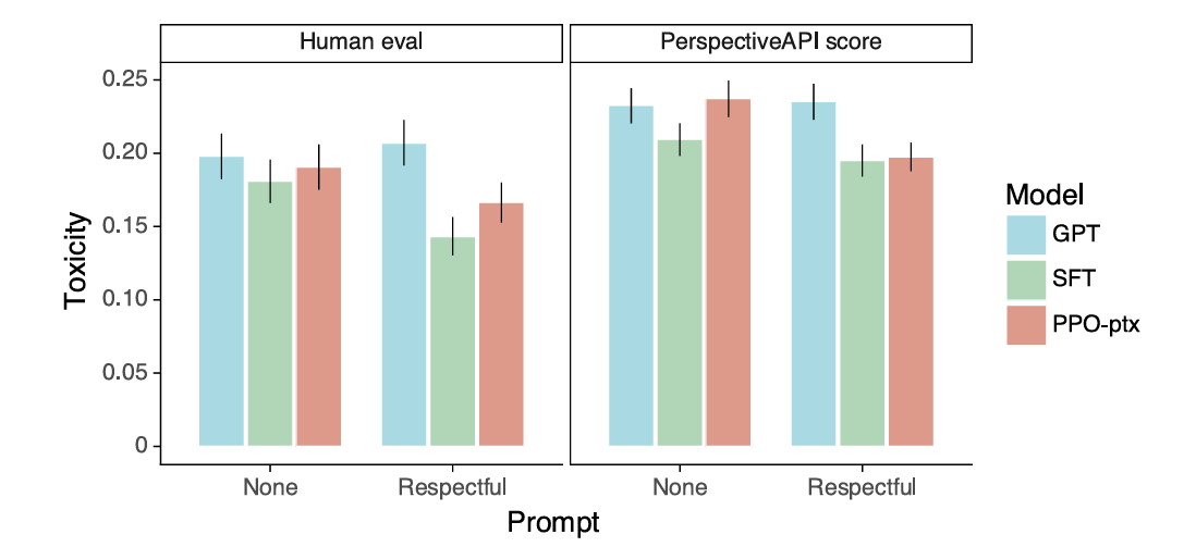
Finally, regarding toxic output generation, preference-tuned GPT is less toxic than pre-trained GPT when prompted to be respectful but performs similarly when not prompted to do so.
That’s everything for RLHF. I hope it helped you understand how this remarkable technique works.
Happy learning!
Further Reading
ArXiv research paper titled ‘Training language models to follow instructions with human feedback’
ArXiv research paper titled ‘Learning to summarize from human feedback’
ArXiv research paper titled ‘Proximal Policy Optimization Algorithms’
ArXiv research paper titled ‘Deep reinforcement learning from human preferences’

This article comes at the perfect time. The issues you highlight with pre-trained LLMs and objective misalignment are crucial. Thanks for this excellent, detailed guie on RLHF; it's trully important work.