A Simple Principle From Noise-Cancelling Headphones Supercharges Transformers Like Never Before
A deep dive into the ‘Differential Transformer’ architecture, learning how it works and why it is such a promising architecture to advance LLMs.


Nearly all popular LLMs today are based on the Decoder-only Transformer architecture.
At the heart of this architecture is the Transformer with its Attention mechanism.
This mechanism weighs the importance of different elements in an input sequence and adjusts their influence on the output using Attention scores.
But Transformers aren’t perfect.
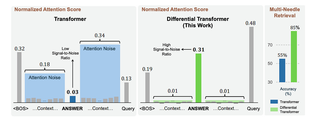
They tend to over-allocate attention to irrelevant context.
Fortunately, we have a new technique that can be applied to the Transformer to fix this issue.
The resulting architecture, called the Differential Transformer, beats the conventional Transformer when the model size and training tokens are scaled.
It is also better than the Transformer at long-context language modelling, key information retrieval, reducing hallucinations, and in-context learning.
Here’s a story in which we deep-dive into this architecture, learning how it works and why it is such a promising architecture for advancing LLMs.
Let’s First Learn About The Decoder-Only Transformer
The original paper on Transformers implemented it using the Encoder-Decoder architecture, which was more suitable for machine translation tasks.
This was soon modified to the Decoder-only Transformer for language modelling tasks, and this architecture has been used in almost all modern-day LLMs since.
A Decoder-only Transformer conventionally consists of multiple stacked layers that consist of:
Causal/ Masked Multi-Head Self-Attention (MHA)
Layer Normalization (Pre-Norm or Post-Norm, depending on whether the inputs are normalized before or after each sub-layer, respectively.)
Feed-Forward Network (FFN)
Residual Connections between the layers that are used to stabilize gradients

The Causal/ Masked Multi-head Self-Attention is at the heart of this architecture, allowing each token to attend only to previous tokens in the sequence.
This ensures the model generates text from left to right without seeing future tokens.
The outputs from this attention mechanism are transformed using Layer Normalization and feed-forward layers.
Finally, the outputs from the last layer of the Transformer (after the top LayerNorm in the image above) are passed through a Linear/ fully connected layer.
This converts these outputs into a vector of size equal to the model's vocabulary size. The values produced are called logits.
A Softmax function converts these logits into a probability distribution over the vocabulary.
The LLM uses this to choose the token at the index with the highest probability (Greedy Decoding) as its next output or uses probabilistic sampling for this purpose, thus generating text autoregressively.
A Deeper Dive Into Attention Calculations
In a traditional Transformer, given a sequence of input token embeddings X, these are first projected into Query (Q), Key (K), and Value (V) matrices using learnable weight matrices.

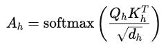
Next, attention scores are calculated using the scaled dot-product as follows, where d is the Query/ Key dimension:

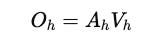
These attention scores are then used to scale the Value (V) matrix as follows:

To ensure that tokens only attend to tokens before them for computing attention, the future tokens are masked. This approach forms the basis of Causal/ Masked Multi-head Self-Attention.
The masked scores are calculated as:

where M represents the mask matrix where M(i)(j) is the element in the mask for position i (Query) attending to position j (Key).
In the matrix, the elements are:
0fori ≥ jwhich means that the tokenican attend to itself and all previous tokens.−∞fori < jwhich means that tokenicannot attend to future tokens

We choose the −∞ because the softmax probability calculated for this term results in 0.
This ensures that the probability assigned to future tokens is zero, creating a mask and preventing the model from attending to them.
The final output is then calculated using the masked scores as follows:

Attention Calculations For Multiple Heads
The Transformer architecture uses multiple heads to calculate multiple Attention scores in parallel.
This helps the architecture capture better semantic relationships between different tokens.
Instead of working with full-dimensional vectors (d(model)), each head works with lower-dimensional projections (d(h)) of the Queries, Keys and Values, where d(h) = d(model) / h.
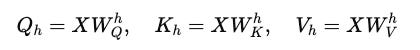
where W(Q)(h), (W)(K)(h), W(V)(h) are weight matrices for each head h.
Each head’s attention score is calculated as:
This score scales the Value matrix, resulting in each head’s output.
Finally, the outputs of all heads are concatenated and transformed as:
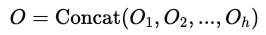
Another weight matrix W(O) transforms the concatenated output back into the original model dimension (d(model)).


The above calculations are shown without the mask, but note that traditional decoder-only architecture contains the Causal or Masked Multi-head Self-attention mechanism.
A mask M can be added to the above attention calculations to represent them more accurately:

Then, the output can be calculated using the following equation (with other equations remaining the same):

Moving On To The Differential Transformer
Similar to a conventional Transformer, a Differential Transformer has a Decoder-only architecture with L stacked layers, where each layer contains:
Causal/ Masked Multi-head Differential Attention (that replaces the conventional self-attention)
Layer Normalization
Feed-Forward Network (with the SwiGLU activation function)
Residual connections (applied after each layer)
Let’s first discuss in more depth how the Differential Attention module (without multiple heads) works, and then we will return to describe the overall architecture.
Given a sequence of input token embeddings X, these are projected into Query, Key, and Value matrices.
The Query and Key matrices are split into two groups, as shown below.

where W(Q), (W)(K), W(V) are weight matrices.
Next, the attention scores are computed separately for both Query-Key pairs:

where d is the dimension of the Query and Key vectors.
Following this, the difference between the two attention scores is computed as follows:


where λ is a learnable scalar.
The Value matrix is then scaled using the obtained results as follows:


In the above equations, λ is defined as follows:

where λ(q1), λ(k1), λ(q2), λ(k2) are learnable vectors.
λ(init) is calculated using the following equation, where l represents the index of the layer:

To make things clear till here, we calculate two attention scores where the first A(1) captures general attention between tokens and the second A(2) captures redundant patterns/ noise.
Subtracting A(2) from A(1) removes the noise that was making the Transformer focus on irrelevant context.
λ is a learnable scalar controlling the balance of this subtraction and how much attention noise is removed.
λ(init) and hence λ has a lower value in the early layers of the Transformer than in the deeper layers. This ensures that stronger noise filtering is applied in the deeper layers.
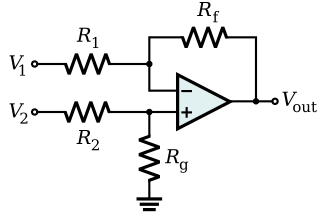
This idea is based on a Differential amplifier, a type of electronic amplifier that amplifies the difference between two input voltages but suppresses any voltage common to them.
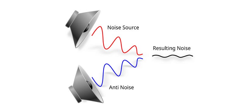
A similar principle applies to noise-cancelling (NC) headphones, which detect external noise and produce an inverted wave similar but opposite to this noise.
Cancellation occurs when the original noise is subtracted using the inverted wave, a process called Destructive interference.
Differential Attention With Multiple Heads
Differential attention is further enhanced by using a multi-head mechanism.
For h number of attention heads, the given sequence of input token embeddings X is projected into two Queries, two Keys and a Value for each head using different learnable projection matrices.
Instead of working with full-dimensional vectors (d(model)), each head works with lower-dimensional projections (d(h)) of the Queries, Keys and Values, where d(h) = d(model) / h.

Next, attention scores are calculated for each head i (from 1 to h) as follows:
Following this, the difference between the two attention scores is computed as follows

The term λ is shared between the heads within the same layer, and computed once per layer (not per head).
The resulting score scales the Value matrix, resulting in each head’s output.

Each head’s output is then normalized using RMSNorm, and scaled using the term (1 − λ(init)).

After computing the outputs for all h heads, they are concatenated and scaled using a matrix W(O).
This concatenation transforms the combined output of all heads back into the original model dimension.


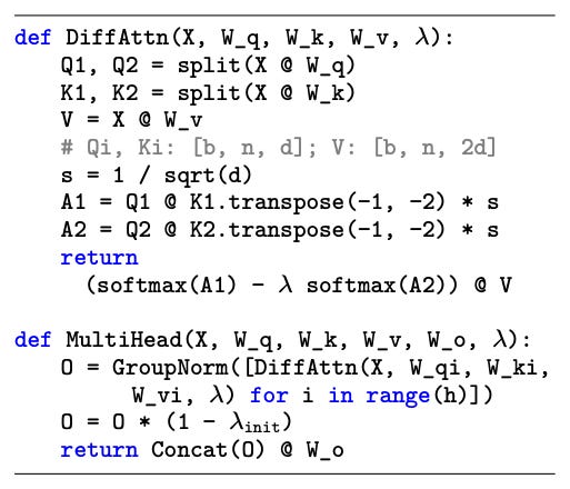
The resulting multi-head Differential attention module is shown in the image below.

The pseudocode for the module is as follows:
The Overall Architecture Of The Multi-Head Differential Transformer
Coming back to what we discussed earlier, the overall Differential Transformer has a Decoder-only architecture with L stacked layers, where each layer contains:
Multi-head Differential attention (now you understand how this works) with a residual connection

where Y(l) is the output of the multi-head differential attention module, within the layer l, X(l) is the input to the layer l, and this added back to Y(l) represents the residual connection
Feed-forward network (FFN) (applying the SwiGLU activation function) with a residual connection

Inspired by LLaMa, RMSNorm Layer Normalization is applied before the Differential Attention and Feed-forward modules.
This approach is termed pre-RMSNorm.
(Compare this with GPT-1 that uses post-layer normalization.)
But Is This Architecture Really Any Good?
Performance On Language Modelling
A 3B Differential transformer LLM with a similar architecture to StableLM-3B-4E1T is trained on 1T tokens for this task.
The resulting model, termed Diff-3B, is then compared to similar-scale conventional transformer-based LLMs as baselines.
When evaluated using LM Eval Harness, Diff-3B reaches better accuracy on multiple benchmarks compared to the baselines.

Scalability
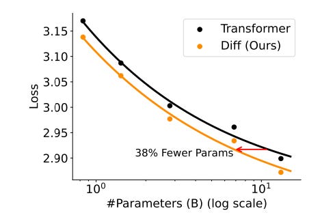
On scaling the model size from 830 to 13B parameters, the LLMs with the Differential transformer outperform the conventional ones for all model sizes.
A 6.8B Differential transformer-based LLM achieves validation loss similar to that of an 11B conventional LLM, using only 62.2% of the parameters!
On scaling training tokens up to 260B, for comparable 3B models, the Differential transformer-based LLM again outperforms the conventional one, achieving higher training data efficiency for all token sizes.
A Differential transformer-based LLM trained on 160B tokens matches the performance of a Transformer-based LLM trained with 251B tokens!

Overall, a Differential transformer-based LLM requires only about 65% of model size or training tokens to match the Transformer-based LLM’s performance.
Performance On Long Context Tasks
When the 3B LLMs are scaled from 4K to 64K context length, the Differential transformer-based LLM has better long-context comprehension and retention than the standard Transformer-based LLM.
This is seen with the lower cumulative average Negative Log-Likelihood (NLL) for the Differential transformer-based LLM, for increasing context length (Lower NLL means better long-context understanding).

Performance On Key Information Retrieval
This evaluation involves testing whether an LLM can find important information (‘needle’) hidden in large amounts of surrounding context (‘haystack’), and therefore called the ‘Needle-In-A-Haystack’ test.
A specific approach to this test, called ‘Multi-needle evaluation,’ involves using multiple ‘needles’ (a unique magic number given to a specific city) hidden at five different depths (0% to 100%) within the context.
The LLMs are then asked to retrieve the correct numbers for the given cities.
For a 4K context length, the Differential Transformer-based LLM maintains high accuracy even as the number of needles increases, unlike the standard Transformer-based LLM, which shows a significant performance drop.

For a 64K context length, the Differential Transformer-based LLM again shows strong results, outperforming the Transformer-based LLM by up to 76% when the needle is placed early in the sequence (at 25% depth).

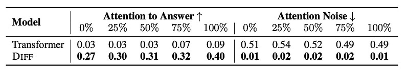
Compared to the conventional LLM, the Differential Transformer-based LLM allocates higher attention scores to the correct answer span and lower attention scores to noise.
This is one reason why it performs so well at key information extraction.
Performance On In-Context Learning
In-context learning occurs when an LLM can perform new tasks by simply analysing the instructions and examples given within the prompt, without updating its parameters.
To test this, 3B LLMs are shown multiple input-output examples in their prompt and asked to classify new inputs (Many-Shot In-Context Learning for classification).
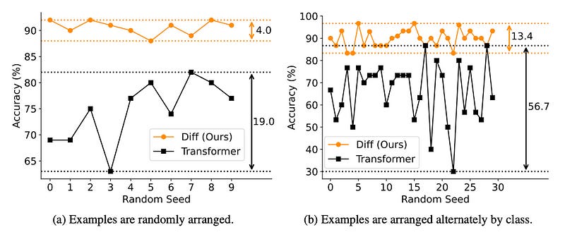
The Differential Transformer-based LLM outperforms the conventional one with gains in average accuracy ranging from 5.2% to 21.6% across multiple classification datasets.

The performance is better and robust even when the order of prompt examples changes.
Hallucinations
The Differential Transformer-based LLM reduces hallucination in both text-summarization and question-answering tasks by better attending to the relevant parts of the input on multiple datasets.


The overall results are very impressive, alongside the fact that the Differential attention mechanism can be easily implemented with FlashAttention, making it even more efficient.
I wouldn’t be surprised to see this architecture soon become the backbone of future LLMs!
What are your thoughts on this? Let me know in the comments below!
Further Reading
Research paper titled ‘Differential Transformer’ published in ArXiv
Code implementation of the Differential Transformer from the original research paper
Research paper titled ‘Attention Is All You Need’ published in ArXiv
Research paper titled ‘Generating Wikipedia by Summarizing Long Sequences’ published in ArXiv
Research paper titled ‘Improving Language Understanding by Generative Pre-Training’ by OpenAI
Source Of Images
All images used in the article are created by the author or obtained from the original research paper unless stated otherwise.