'FANformer' Is The New Game-Changing Architecture For LLMs
A deep dive into how FANFormer architecture works and what makes it so powerful compared to Transformers


LLMs have always surprised us with their capabilities, with many speculating that scaling them would lead to AGI.
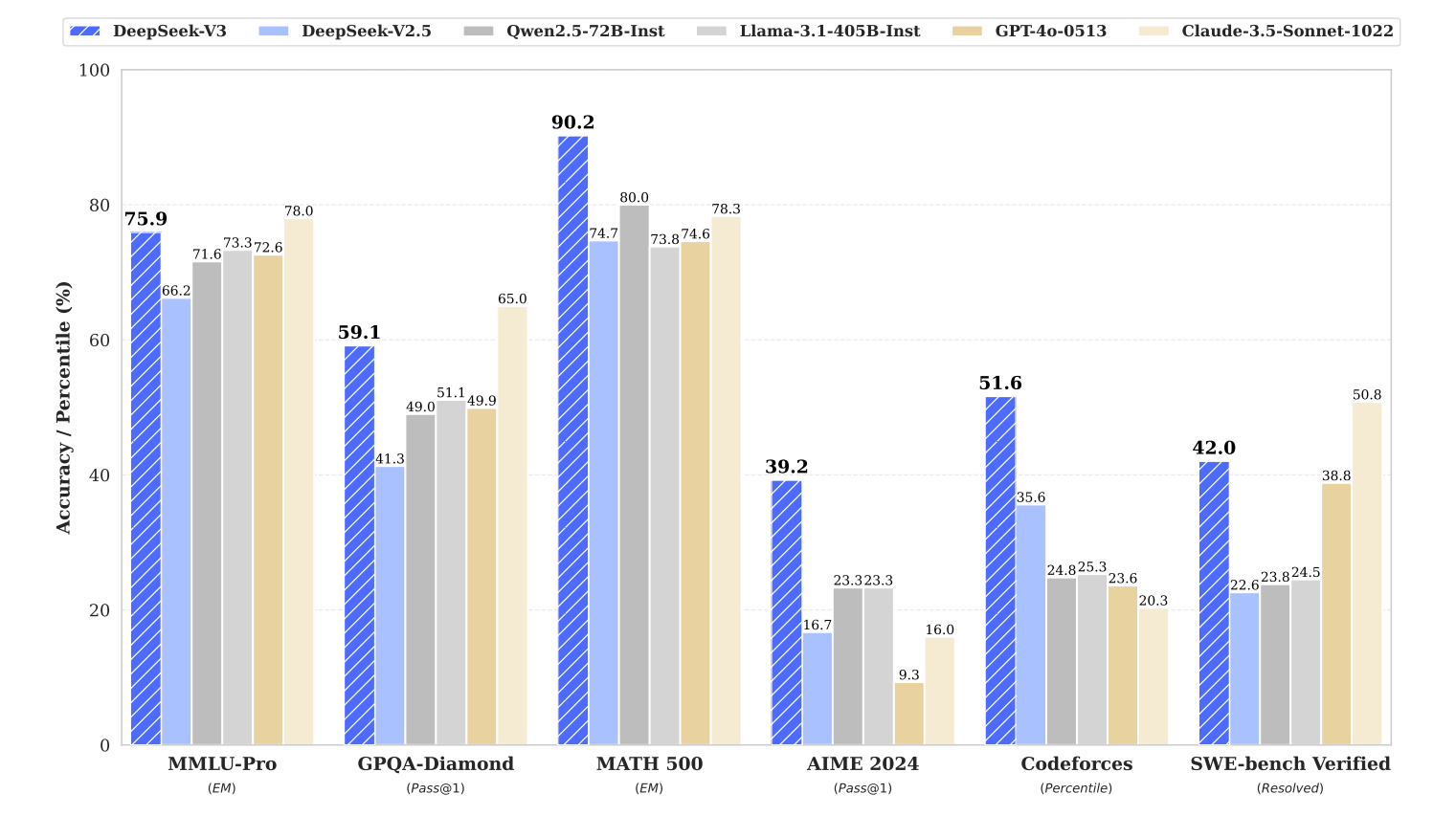
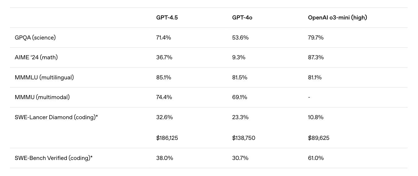
But such expectations have led to disappointments in the last few days, with GPT-4.5, the largest and best model for chat from OpenAI, performing worse than many smaller models on multiple benchmarks.
While DeepSeek-V3 scores 39.2% Pass@1 accuracy on AIME 2024 and 42% accuracy on SWE-bench Verified, GPT-4.5 scores 36.7% and 38% on these benchmarks, respectively.
This raises the question: Do we need a better LLM architecture to scale further?
Luckily, we have a strong candidate that has been put forward by researchers recently.
Called FANformer, this architecture is built by combining the powerful Fourier Analysis Network (FAN) into the Attention mechanism of Transformers.
The results of experiments performed with them are very promising, with FANformers consistently outperforming Transformer when scaling up model size and training tokens.
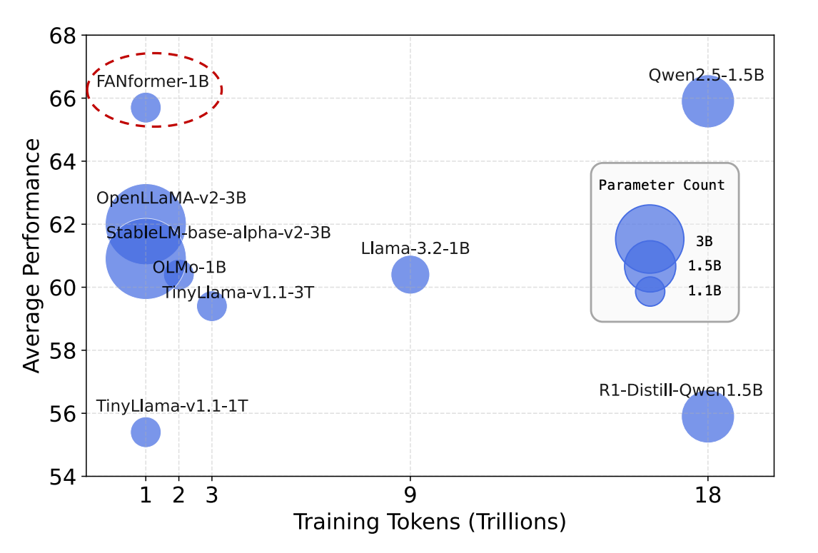
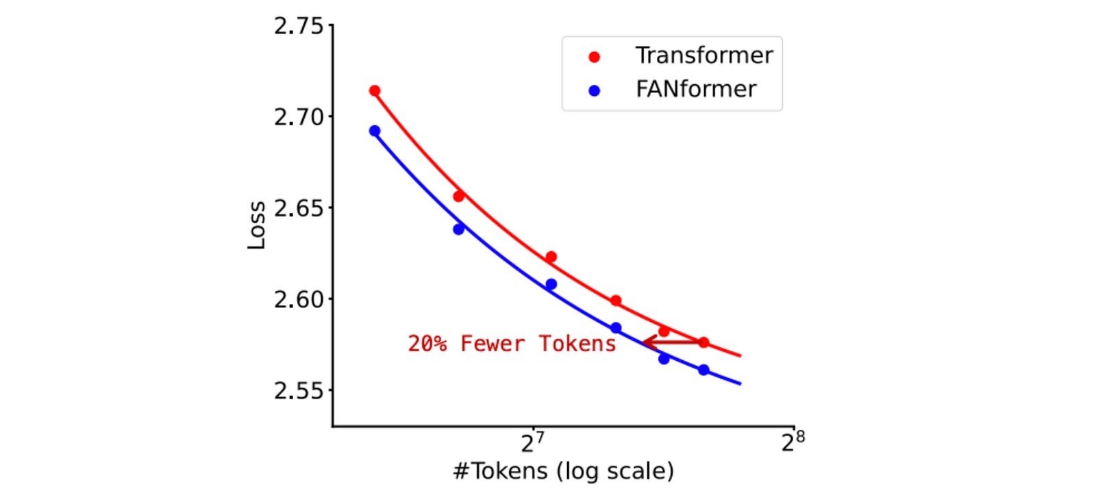
As seen in the plot below, a FANformer with 1 billion parameters performs better than other open-source LLMs of comparable size and training tokens.
Here’s a story where we deep dive into how a FANFormer works and discuss all the architectural modifications that make it so powerful.
Let’s begin!
We Begin With ‘Fourier Analysis Networks’
Standard deep neural networks/ MLPs do very well at capturing and modelling (“learning”) most patterns from training data, but there’s one domain where they largely fall short.
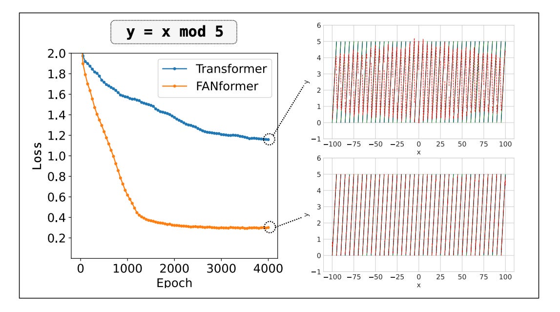
This is — Modelling Periodicity in data.
Since most data contain hidden periodic patterns, this hinders the learning efficiency of traditional neural networks.
Check out the following example where a Transformer struggles to model this simple mod function even when given sufficient training resources.
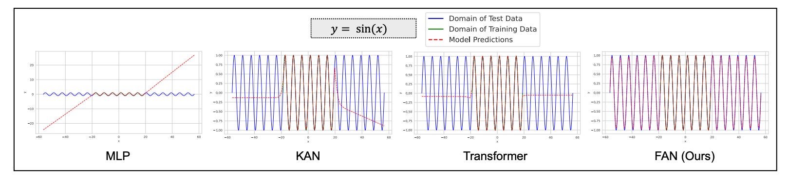
This is fixed by Fourier Analysis Networks (FANs), which use the principles of Fourier Analysis to encode periodic patterns directly within the neural network.
This can be seen in the following example, where a FAN can better model a periodic sin function compared to MLP, KAN and Transformer.
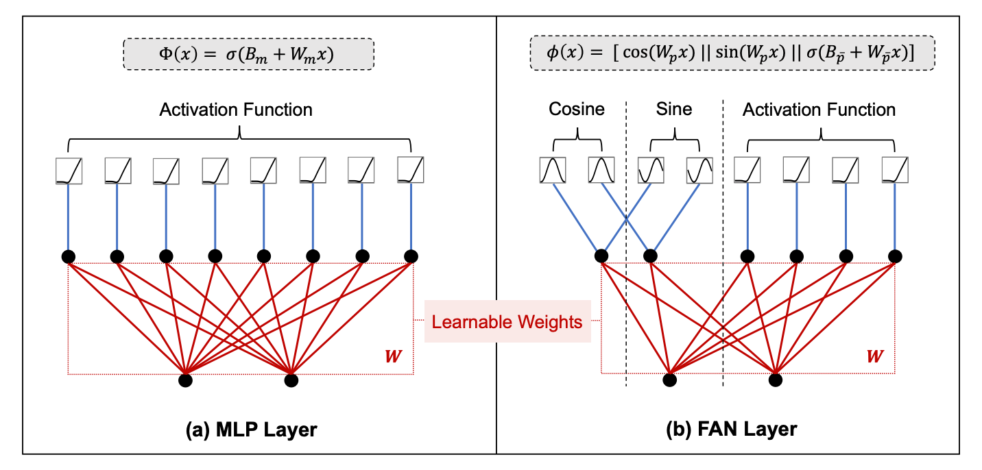
A FAN Layer is described using the following equation:

where:
Xis the inputW(p)andW(p̄)are learnable projection matricesB(p̄) is the bias termσrepresents a non-linear activation function||denotes concatenation
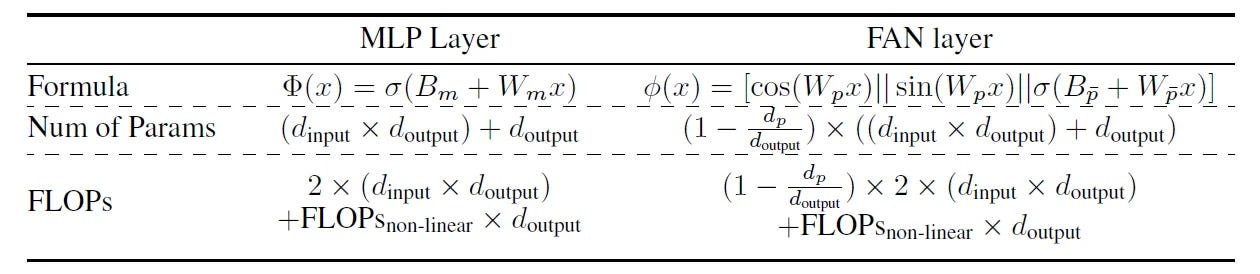
Compared to an MLP layer that applies a simple linear transformation followed by a non-linear activation, the FAN layer explicitly integrates periodic transformations (sine and cosine) with the linear transformation and non-linear activation.

This helps a FAN layer capture periodic patterns in the input data alongside its general-purpose modelling capabilities.
Here’s a visual and mathematical comparison between MLP and FAN layers.
If you’d like to learn about FANs in more depth, here’s one of my lessons on how they work and how to code one from scratch.

Moving Forward To Building The Attention Mechanism Of A FANformer
Most popular LLMs today have a decoder-only Transformer architecture.
A FANformer borrows the periodicity-capturing principles from FAN and applies them to the Attention mechanism of this Transformer architecture.
This revised Attention mechanism is called the ATtention-Fourier (ATF) module.
Given an input sequence s of length l, represented by s = { s(1), s(2), …, s(l) }, it is first mapped to an input embedding X(0) where X(0) = { x(1), x(2), …, x(l) }.
This embedding passes through the layers of a model, obtaining the final output X(N), where N is the total number of layers in the model.
Let’s learn how each layer processes the embedding.
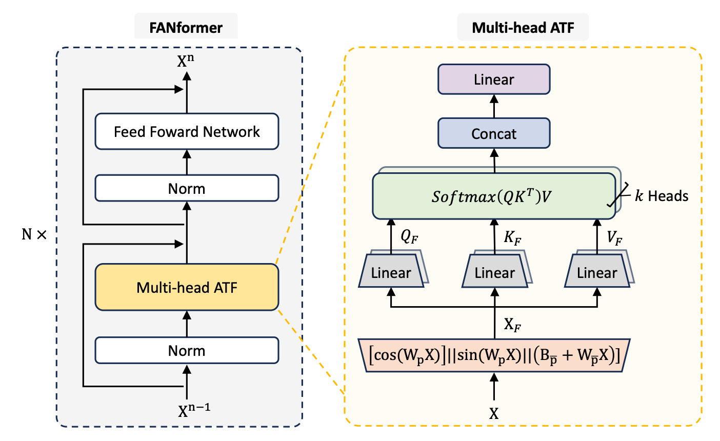
Given an input embedding X, its Fourier-transformed representation is first computed as:

As you will notice, this transformation uses a slightly modified FANLayer’ where the activation function σ in the original FANLayer equation is simply replaced by an identity function or σ(x) = x.
Next, linear transformations are applied to the output X(F) to compute the query (Q), key (K), and value (V) as shown below:

where W(Q), W(K), and W(V) are learnable weight matrices used to compute the query (Q), key (K), and value (V), respectively.
Following this, the scaled dot-product attention is calculated using the Fourier-transformed Q, K, and V as follows:

where d(h) is the model’s hidden dimension.
Note that ATF(X) is mathematically equivalent to Attention(FANLayer′(X)), because the Fourier transformations do not alter the attention mechanism itself but only how input representations are computed.
This makes it possible to use advanced architectures like FlashAttention with the FANLayer', and therefore, with the FANFormer.
Building Up To Multi-Head ATF
The attention module is further extended to multiple heads, similar to traditional Multi-head Attention.
For a given input X, it is first projected into k independent heads using the previously described ATF module as follows:

where for the i-th head:
W(Q)(i),W(K)(i),W(V)(i)are the learnable weight matrices for each head’s (Q(i)), key (K(i)), and value (V(i)), respectively, calculated as follows:

d(k)is the dimension per head when usingkattention heads, calculated as= d(h) / kwhered(h)is the model’s hidden dimension.
Then, the outputs of all the heads are concatenated and linearly transformed using an output weight matrix (W(O)).

The FANformer architecture is shown in the illustration below.
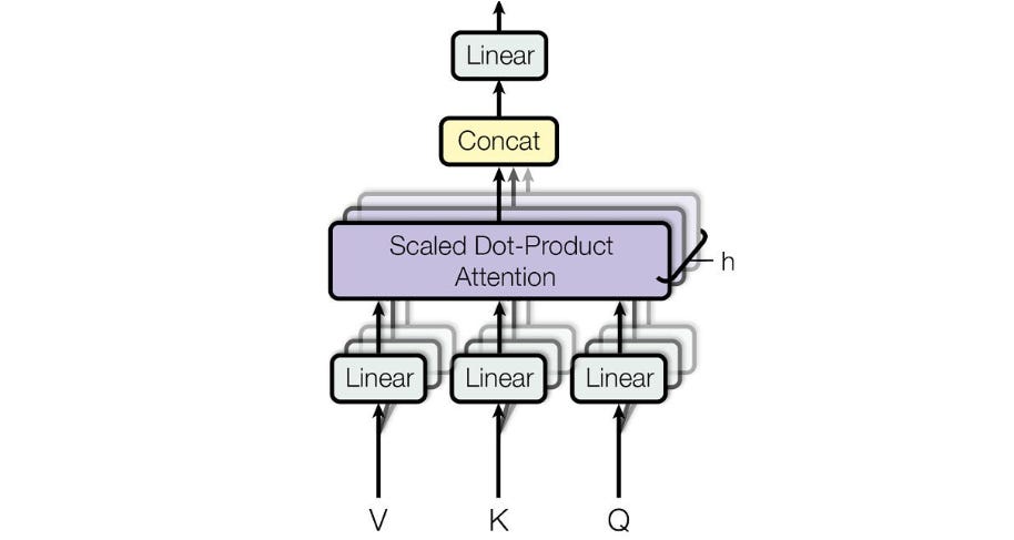
Compare it with the conventional Multi-head Attention shown below, where Q, K and V for each head are computed directly from the input embedding without any Fourier transformation.
The pseudocode for the Multi-head ATF is shown below:
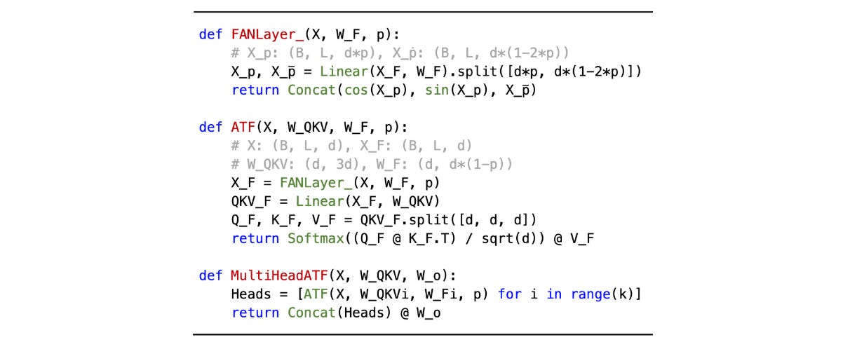
Note that in the above, p is the hyperparameter that controls how much of the input X is processed through the periodic (X_p) vs. non-periodic components (X_p̄) following the FANLayer’ equation.
p is set to 0.25 by default in the experiments.
Stacking Up To A FANformer
A FANformer is built by stacking N FAN-former layers where each layer consists of:
a Multi-head ATF (Attention-Fourier) module
a Feedforward Network (FFN) module
The Multi-head ATF output is calculated based on the previous equation:
But the input for each layer (X(n)) is modified using Pre-Normalization (Pre-Norm) and then adding the original input back to the computed output from the MultiHeadATF.

Y(n) is then transformed using the Feedforward Network (FFN) module as follows:

where FFN uses the SwiGLU activation as follows:

where W(1), W(2), and W(3) are learnable weight matrices and ⊗ denotes element-wise multiplication.
Reading these equations with the visual representation of the FANformer side by side is highly encouraged to understand them better.
How Good Is The FANFormer?
Researchers construct a FANformer by integrating the ATF module into the open-source LLM, OLMo, using it as the baseline Transformer.
Tokens are sampled from OLMo’s training data, called Dolma, and used to pre-train FANformers of different sizes.
Scaling Experiments
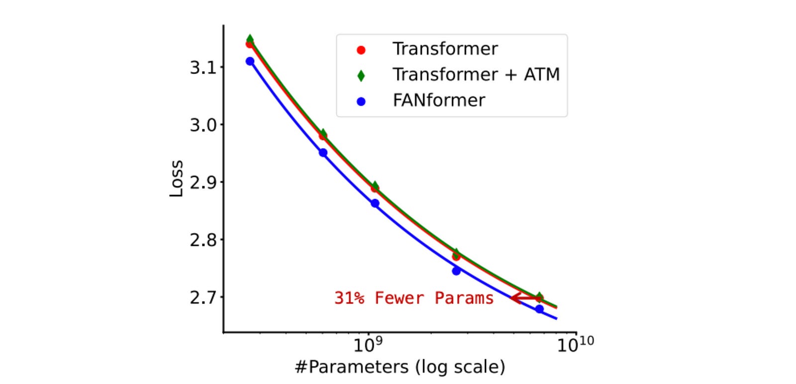
On scaling experiments, the FANformer consistently outperforms the standard Transformer across all model sizes and achieves comparable performance while using only 69.2% of its parameters!
The scaling curve for a variant of FANformer called Transformer + ATM, which uses MLP layers instead of FAN layers, is very similar to that of a standard Transformer.
This shows that the revised attention mechanism with MLP layers is not as good, and instead, the periodicity capturing architectural changes is what gives the FANformer real performance boost.
Further experiments show that the FANformer requires 20.3% fewer training tokens to match the performance of the standard Transformer.
Performance On Downstream Tasks
FANformer’s zero-shot performance is compared with 7 open-source LLMs (of similar size/ training tokens) on a set of 8 downstream tasks using the following benchmarks:
BoolQ (Boolean question answering)
HellaSwag (Commonsense completion)
OBQA (Open book question answering)
PIQA (Physical reasoning)
SCIQ (Science question answering)
WinoGrande (Co-reference resolution)
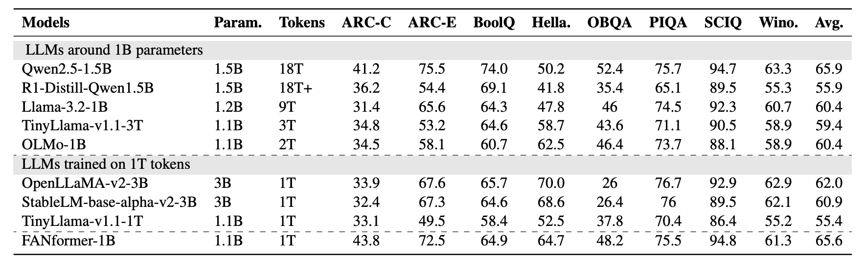
Experiments show that FANformer-1B consistently outperforms other LLMs with similar parameter counts while requiring significantly less training data.
Notably, FANformer-1B's performance is comparable to Qwen2.5–1.5B, the current state-of-the-art LLM around the 1 billion parameter mark.
Also, R1-Distill-Qwen1.5B, a model distilled from DeepSeek-R1 with strong reasoning capabilities, cannot outperform the FANformer on most non-reasoning commonsense tasks.
This shows how important pre-training is and that distillation alone is not enough for strong model performance on downstream tasks.
Training Dynamics
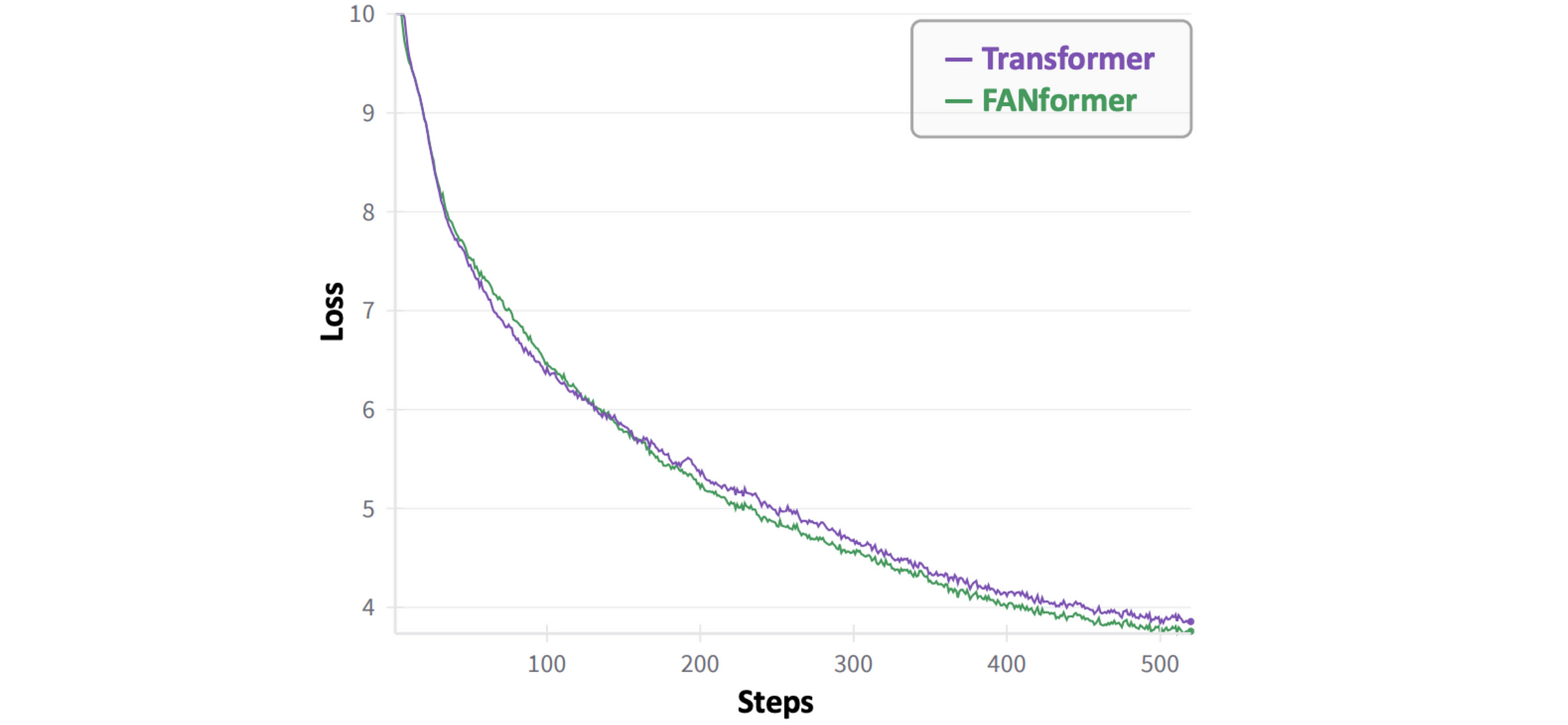
In the early stages of training, the FANformer’s loss decreases more slowly than that of the standard Transformer’s.
This could be because the model has not learned to recognize the periodic patterns in the data in its early stages.
But as the training progresses, the FANformer converges faster than the Transformer.
Instruction Following Performance with Supervised Fine-Tuning (SFT)
The pretrained FANformer-1B model is further supervised fine-tuned on the tulu-3-sft-olmo-2-mixture dataset (following OLMo), leading to FANformer-1B-SFT.
Similarly, OLMo-1B-SFT, the 1 billion parameter version of OLMo is supervised fine-tuned on the same dataset.
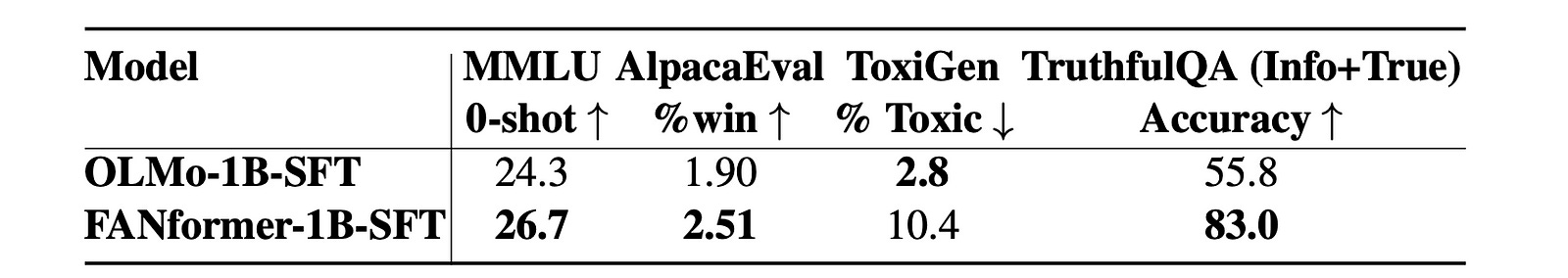
These models are evaluated using four benchmarks as follows:
MMLU (General knowledge and reasoning)
TruthfulQA (Truthfulness & informativeness)
AlpacaEval (Instruction-following quality)
ToxiGen (Toxicity filtering capability)
Results again show the superior performance of FANformer-1B-SFT on MMLU, AlpacaEval, and TruthfulQA compared to OLMo-1B-SFT.
Filling A “Hole” In Mathematical Reasoning
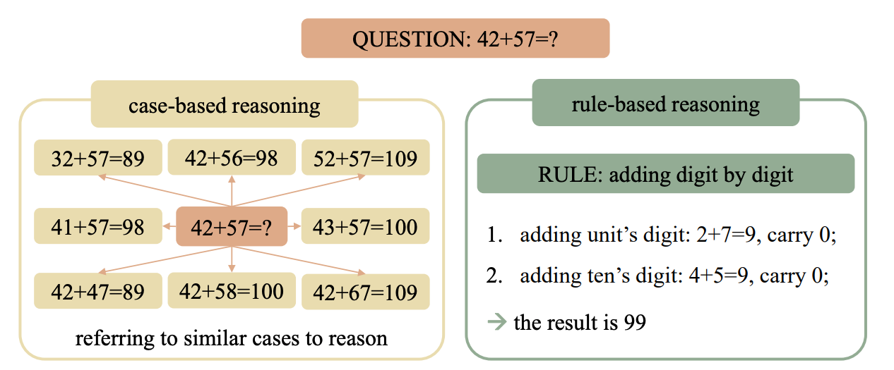
A 2024 research paper described how Transformer-based LLMs use Case-based reasoning to solve mathematical problems.
This means that they memorize specific examples from training data and then try to generalize by finding similar cases during inference.
This differs from Rule-based reasoning, which involves learning underlying mathematical rules and applying them systematically for problem-solving.
But do FANformers solve maths this way as well?
To test this, OLMo-1B and FANformer1B, are evaluated on two mathematical problems:
Modular Addition: Solve
c = (a + b) mod 113witha, b ∈ [0, 112]Linear Regression: Solve
c = a + 2b + 3witha, b ∈ [0, 99]
They are fine-tuned on each task dataset, and their performance is measured via the Leave-Square-Out method.
This is where a square region of data points is removed from the training set, and the model is trained on the remaining data to ensure that it is not exposed to the left-out square region.
The model’s performance on these left-out data points is then evaluated during testing.
In experiments, both architectures achieve near-perfect accuracy on the training dataset. However, Transformers fall short on the test dataset.
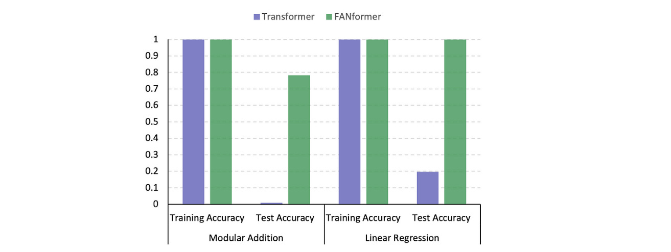
Transformer shows a “black hole” pattern in Leave-Square-Out testing, where its accuracy drops to nearly zero on unseen data, confirming that it might not be using rule-based reasoning for mathematical problem-solving.
However, tests on FANformer tell something different.
No obvious “black hole” is seen in the test figures, which tells that they learn the underlying mathematical rules for problem-solving and, thus, perform better.

It’s surprising how explicitly encoding periodicity-capturing capabilities in the deep neural network/ Transformer architecture can make it so powerful.
Although many further experiments on FANformers are required, it would be exciting to see them used in the powerful LLMs of the future.
Further Reading
Research paper titled ‘FAN: Fourier Analysis Networks’ published in ArXiv
Research paper titled ‘OLMo: Accelerating the Science of Language Models’ published in ArXiv
Source Of Images
All images are obtained from the original research paper unless stated otherwise.