

Kolmogorov-Arnold Networks (KANs) Are Being Used To Boost Graph Deep Learning Like Never Before
A deep dive into how Graph Kolmogorov-Arnold Networks (GKANs) are improving Graph Deep Learning to surpass traditional approaches


KANs have gained a lot of attention since they were published in April 2024.
They are being used to solve several machine-learning problems that previously used Multi-layer Perceptrons (MLPs), and their results have been impressive.
A team of researchers recently used KANs on Graph-structured data.
They called this new neural network architecture — Graph Kolmogorov-Arnold Networks (GKANs).
And, how did it go — you’d ask?
They found that GKANs achieve higher accuracy in semi-supervised learning tasks on a real-world graph dataset (Cora) than the traditional ML models used for Graph Deep Learning, i.e. Graph Convolutional Networks (GCNs).
This is a big step for KANs!
Here is a story where we dive deep into GKANs, learn how they are used with graph-structured data, and discuss how they surpass traditional approaches in Graph Deep Learning.
But First, What Is Graph Deep Learning?
Graphs are mathematical structures that consist of nodes (or vertices) and edges (or links) connecting these nodes.
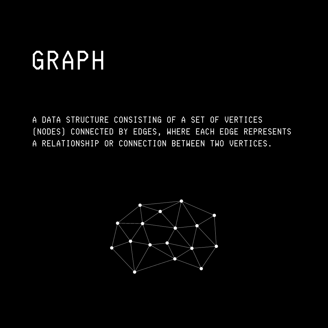
Some examples of real-world data that is structured in the form of graphs include:
Social network connections (Users as nodes and relationships as edges)
Recommendation systems (Items as nodes and user interactions as edges)
Chemical Molecules and compounds (Atoms as nodes and bonds as edges)
Biological molecules such as Proteins (Amino acids as nodes and bonds as edges)
Transportation networks like Roadways (Intersections as nodes and pathways as edges)
Graph Deep Learning is a set of methods developed to learn from such graph-structured data and solve problems based on this learning.
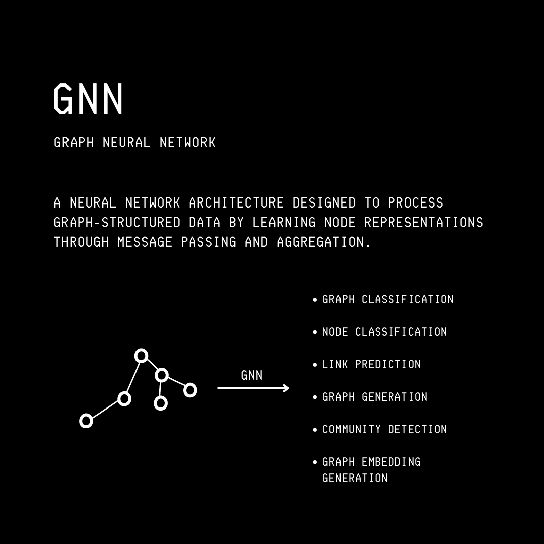
Some of these Graph Learning problems involve:
Graph classification (labelling a graph according to its properties)
Node classification (predicting the label of a new node)
Link prediction (predicting the existence of relations/ edges between nodes)
Graph generation (creating new graphs based on existing ones)
Community detection (identifying clusters of densely connected nodes within a graph)
Graph Embedding generation (generating low dimensional representations of higher dimensional graphs)
Graph clustering (grouping similar graph nodes together)
Graph anomaly detection (figuring out abnormal nodes or edges that do not match the expected pattern in a graph)
Traditionally, these problems have been solved using Graph Neural Networks (GNNs) and their variants (notably Graph Convolutional Networks), which use MLPs at their core.
Let’s explore Graph Convolutional Networks (GCNs) in a bit more detail.
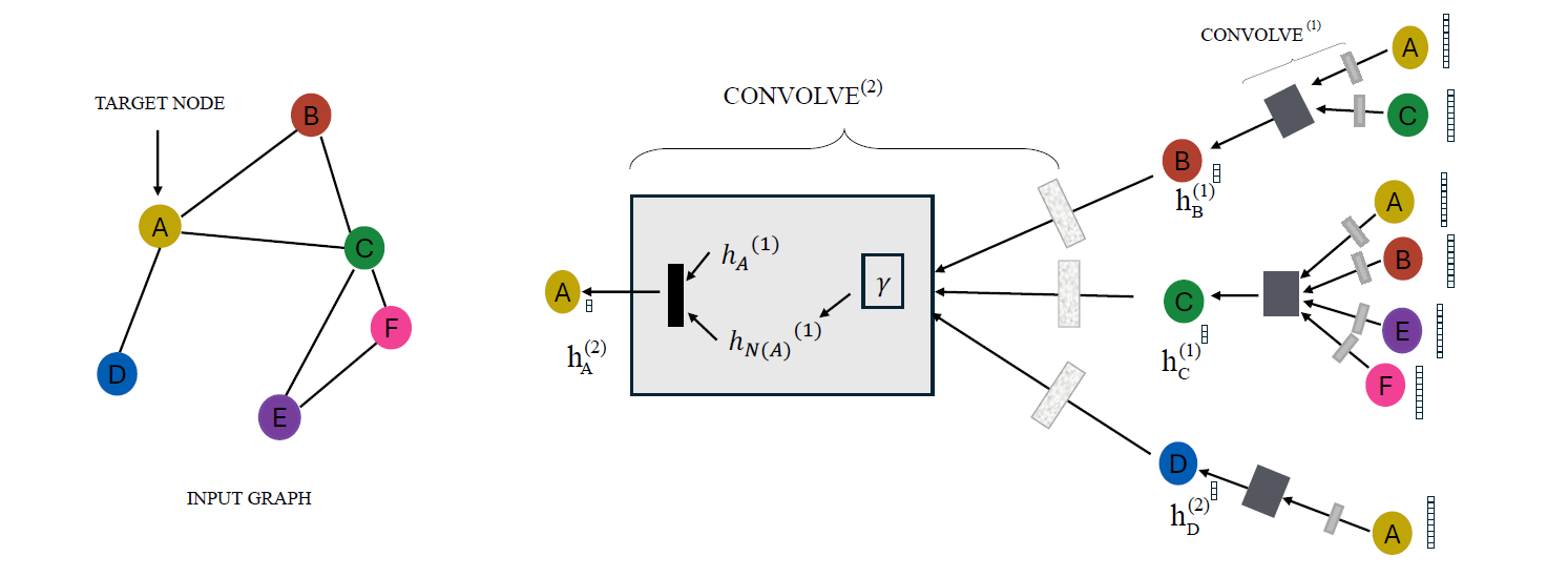
What Are Graph Convolutional Networks?
A Graph Convolutional Network (GCN) combines a graph’s node features with its topology (or how the nodes are connected in space). This allows it to effectively capture the dependencies and relationships in the graph.
In other words, GCNs are based on the assumption that node labels y are mathematically dependent on both the node features X and the graph’s structure (i.e. its adjacency matrix A).
This can be mathematically expressed as:
y = f (X, A)
A multi-layer GCN updates the node representations by aggregating the information from neighbouring nodes using a layer-wise propagation rule:

where:
à = A + Iis the Augmented adjacency matrix or the graph's adjacency matrix with added self-connections for each node. It is the sum of the graph’s adjacency matrix with its identity matrixI.D~is a diagonal matrix ofÃwhere each diagonal element represents the degree of nodeiin the augmented graphD~^(-1/2) à D~^(-1/2)is used to symmetrically normalizeÃ, to make sure that each node’s influence is appropriately scaled by its degree. This normalized adjacency matrix is usually represented withÂ.H(l)is the matrix of node features at layerlH(0)represents the initial node features (orX)W(l)is the trainable weight matrix at layerlσrepresents an activation function (e.g. ReLU)
A simple two-layer GCN’s forward propagation (used for node classification) can be expressed as follows:

where:
Âis the normalized adjacency matrixXis the input feature matrixW(0)andW(1)are the weight matrices for the first and second layers, respectively. These weights are optimized using Gradient Descent.
Now that we know about GCNs let’s move on to learning about KANs.
Next, What Are KANs?
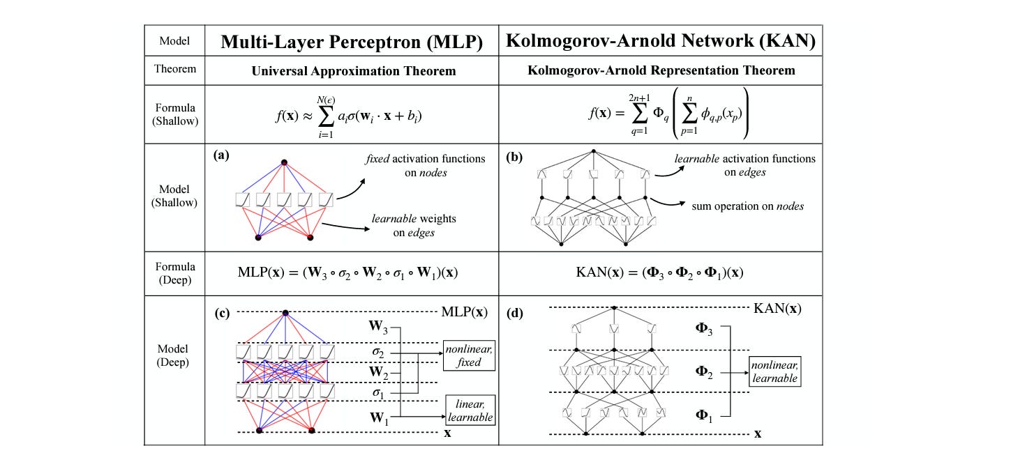
Kolmogorov-Arnold Network (KAN) is a novel and innovative neural network architecture based on the Kolmogorov-Arnold representation theorem.
They are a promising alternative to the currently popular MLPs that are based on the Universal Approximation Theorem.
The core idea behind KANs is to use learnable univariate activation functions (shaped as a B-Spline) on the edges and simple summations on the nodes of a neural network.
This contrasts with MLPs that use learnable weights on the edges while having a fixed activation function on the neural network nodes.
When compared with MLPs, KANs:
Lead to smaller computational graphs
Are more parameter-efficient and accurate
Converge faster and achieve lower losses
Have steeper scaling laws
Are highly interpretable
On the contrary, given the same number of parameters, they take longer to train compared to MLPs.
The Birth Of GKANs
Considering the advantages that KANs offer, researchers devised a novel hybrid architecture called Graph Kolmogorov-Arnold Networks (GKANs) that extended the use of KANs on graph-structured data.
They aimed to find out if GKANs could effectively learn from both labelled and unlabeled data in a semi-supervised setting and outperform traditional graph learning methods.
The team developed two GKAN architectures, which are described below.
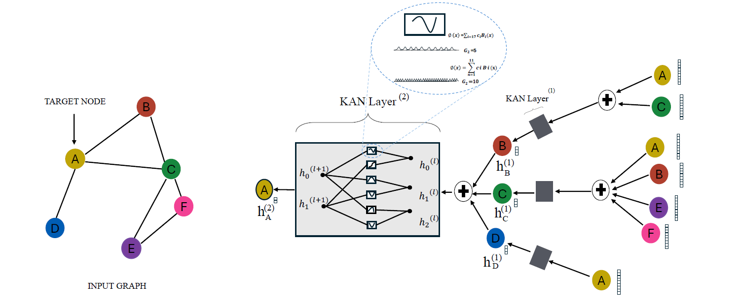
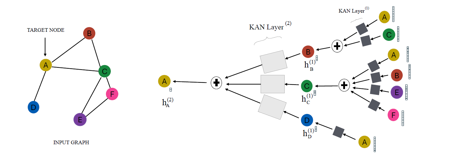
GKAN Architecture 1: Activations After Summation
In this architecture, the learnable univariate activation functions are applied to the aggregated node features after the summation step.
In other words, the node embeddings are first aggregated using the normalized adjacency matrix, and then they are passed through the KAN layer.
The layer-wise propagation rule for GKAN Architecture 1 is shown below.
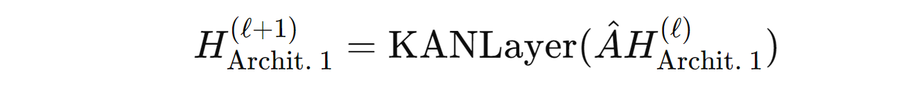
where:
H(l)andH(l+1)represent the node feature matrix at layerslandl+1, respectivelyÂis the normalized adjacency matrixthe
KANLayeroperation applies learnable univariate activation functions or B-Splines to the aggregated node featuresÂH(l)
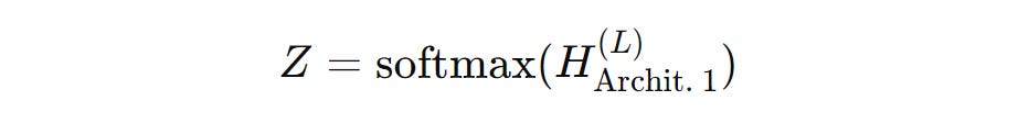
The forward propagation model for the architecture is expressed as:
GKAN Architecture 2: Activations Before Summation
In this architecture, the learnable univariate activation functions are applied to the aggregated node features before the summation step.
In other words, the node features are first passed through the KAN layer and then summated using the normalized adjacency matrix.
The layer-wise propagation rule for GKAN Architecture 2 is shown below.

where:
H(l)andH(l+1)represent the node feature matrix at layerslandl+1, respectivelyÂis the normalized adjacency matrixthe
KANLayeroperation applies learnable univariate activation functions or B-Splines to each element of the input node featuresH(l)
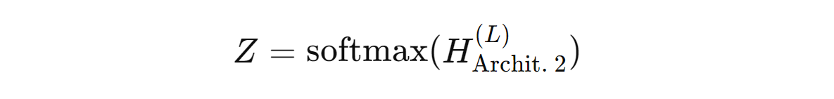
The forward propagation model for the architecture is expressed as:
The Performance Of GKANs
GKANs vs. GCN
Both GKAN architectures were first trained on the Cora dataset.
The Cora dataset is a citation network that consists of documents as nodes and the citation links between these documents as edges.
There are 7 different classes in this dataset that have 1433 features per document.
Next, their performance was compared to that of a conventional GCN, with a comparable number of parameters, over both train and test data using a subset of 200 features from the total 1433 available in the dataset.
And the results were quite incredible!
GKANs achieved higher accuracy than GCNs for both 100 and 200 feature sets.
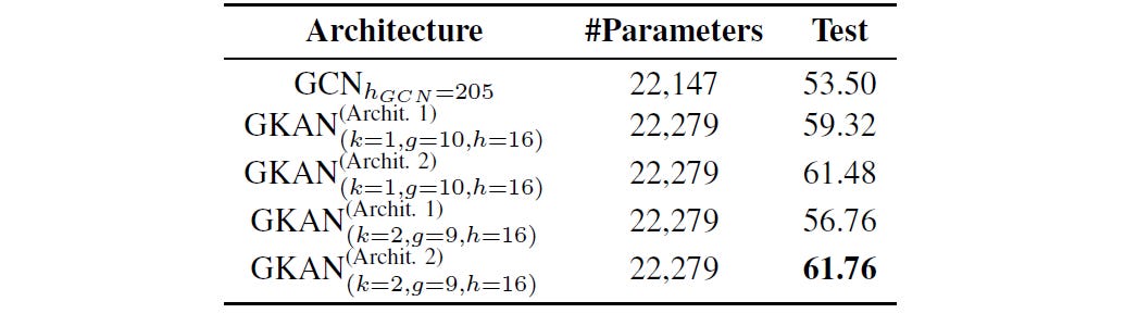
On the first 100 features of the dataset, both GKAN architectures achieved higher accuracy than the GCN.
Notably, the GKAN Architecture 2 achieved 61.76% accuracy compared to 53.5% for GCN.
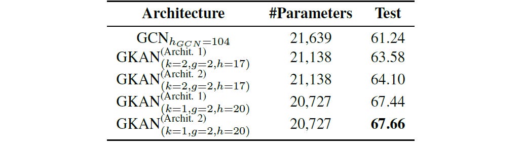
Similarly, both GKAN architectures achieved higher accuracy than the GCN on the first 200 features of the dataset, with the GKAN Architecture 2 achieving 67.66% accuracy compared to 61.24% for GCN.
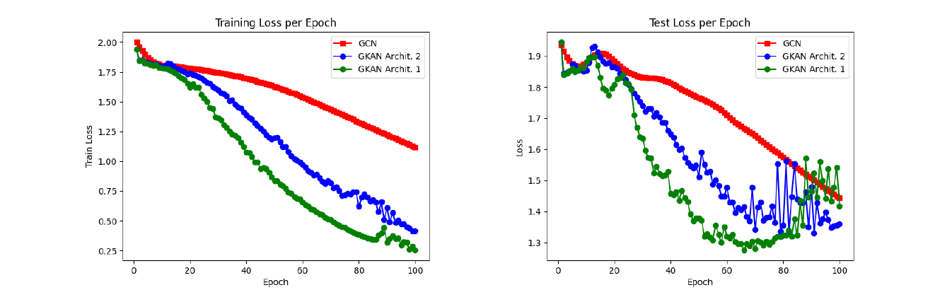
The training and test accuracy plots below showed that GKANs achieved higher accuracy during both the training and testing phases.
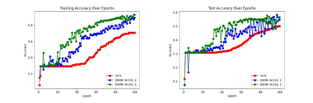
It was also noted that GKAN architectures showed a sharper decrease in loss values during training and required fewer epochs to be trained.
Influence Of Parameters on GKANs
Researchers also evaluated how different parameters impacted the performance of GKANs.
These parameters were:
k: the degree of the polynomial in the spline functionsg: the grid size for the spline functionsh: the size of hidden layers in the network
It was found that the following led to the most effective GKANs.
Lower polynomial degrees (
k = 1out of{1, 2, 3})Intermediate grid sizes (
g = 7out of{3, 7, 11})Moderate hidden layer sizes (
h = 12out of{8, 12, 16})
Training Time
Although GKANs showed high accuracy and better efficiency with faster convergence, researchers noted that their training process was relatively slow, requiring future optimizations.
KANs have opened up a new avenue for improved graph learning and could also be a promising alternative for other graph learning approaches (including Graph Autoencoders, Graph Transformers, and more) that use MLPs at their core.
What are your thoughts on them? Have you used KANs in your projects yet? Let me know in the comments below!
Further Reading
Research paper titled ‘GKAN: Graph Kolmogorov-Arnold Networks’ on ArXiv
Software implementation of GKANs on GitHub (yet to be publically released by the research team)
GitHub repository featuring a curated list of projects using Kolmogorov-Arnold Networks (KANs)