Proximal SFT: SFT Supercharged By RL Is Here

Deep dive and learn about Proximal SFT, a new algorithm that combines SFT with PPO, leading to improved post-training performance of LLMs compared to conventional SFT.

Image generated using Google ImageFX

Supervised fine-tuning (SFT) is the backbone of post-training LLMs today.

Most post-training pipelines begin with SFT, which helps pre-trained LLMs to get better at domain-specific tasks.

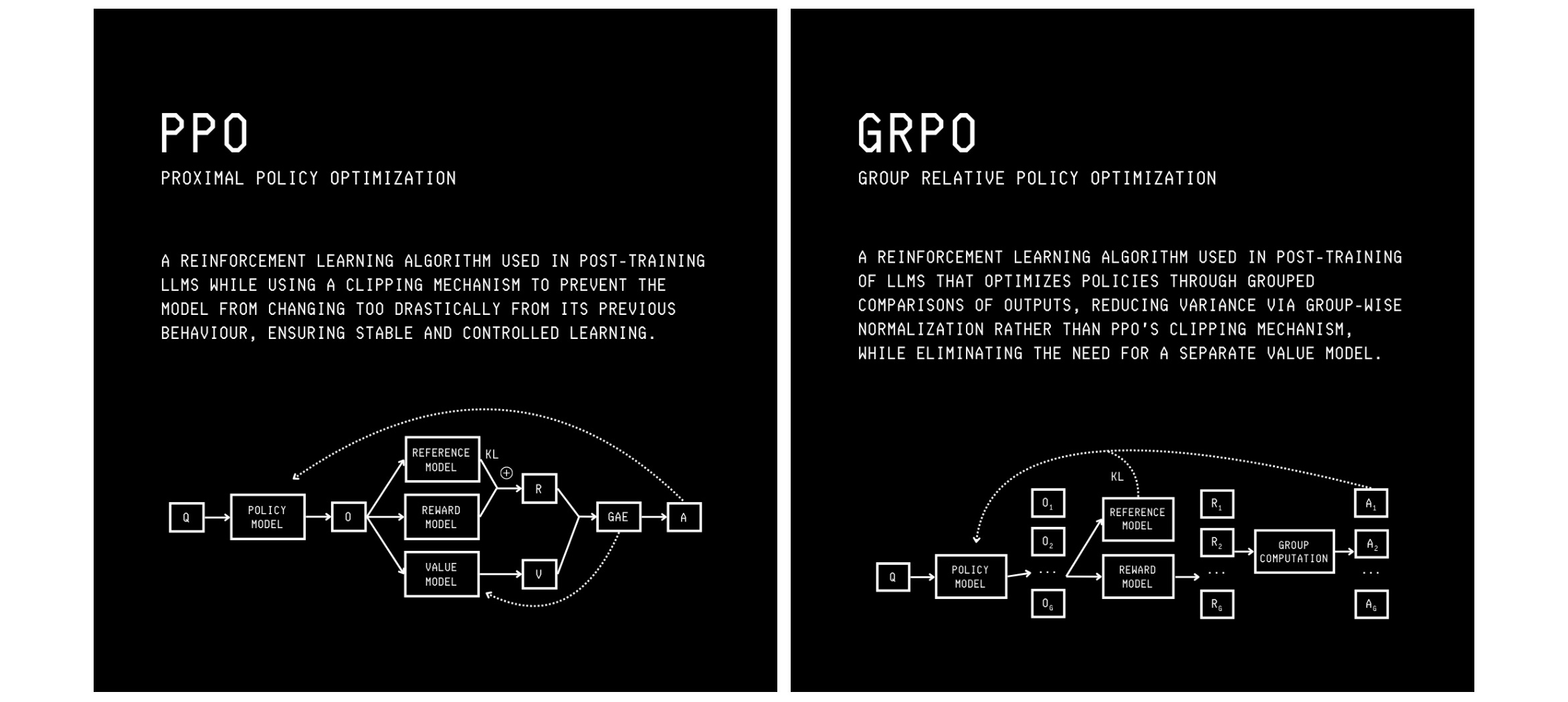
Following SFT, LLMs are aligned with human values (RLHF) or trained to reason better, using PPO or GRPO.

Although post-training with SFT is straightforward and more efficient compared to RL, LLMs trained using it tend to have poor generalization capabilities (i.e., they memorize the training dataset).

Supervised fine-tuned models also show diminished exploration capabilities when further post-trained with RL.

To fix these issues in SFT, researchers have borrowed inspiration from RL algorithms and recently introduced Proximal Supervised Fine-Tuning (PSFT).

This algorithm supercharges SFT by stabilizing the optimization it brings to the model parameters. This leads to better generalization capabilities in an LLM while leaving room for further exploration and improvement in subsequent RL post-training stages.

Here is a story where we deep dive into how Proximal Supervised Fine-Tuning (PSFT) combines SFT and PPO to create an objective that leads to improved post-training performance of LLMs compared to conventional SFT.

Let’s begin!

(Note that this article might be slightly challenging to read for beginners. Rather than being discouraged by it, read it slowly, re-read it multiple times, take your time to understand the equations, and follow all the attached links. If you do so, I promise that you will understand it well and learn something new today.)

---

But First, How Does Supervised Fine-Tuning Work?

Supervised Fine-tuning (SFT) is most commonly the first step when post-training an LLM.

Evolution of different post-training techniques for LLMs (Image from ArXiv research paper titled ‘A Survey on Post-training of Large Language Models’)

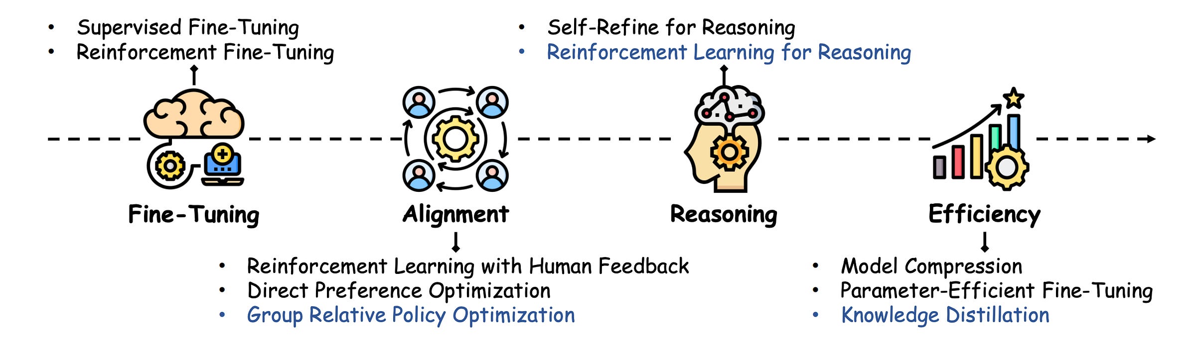
It involves further training a pre-trained LLM on a domain-specific dataset of prompt-response pairs to teach it how to follow instructions and produce desired responses.

Supervised Fine-tuning (Image from author’s book titled ‘LLMs In 100 Images’)

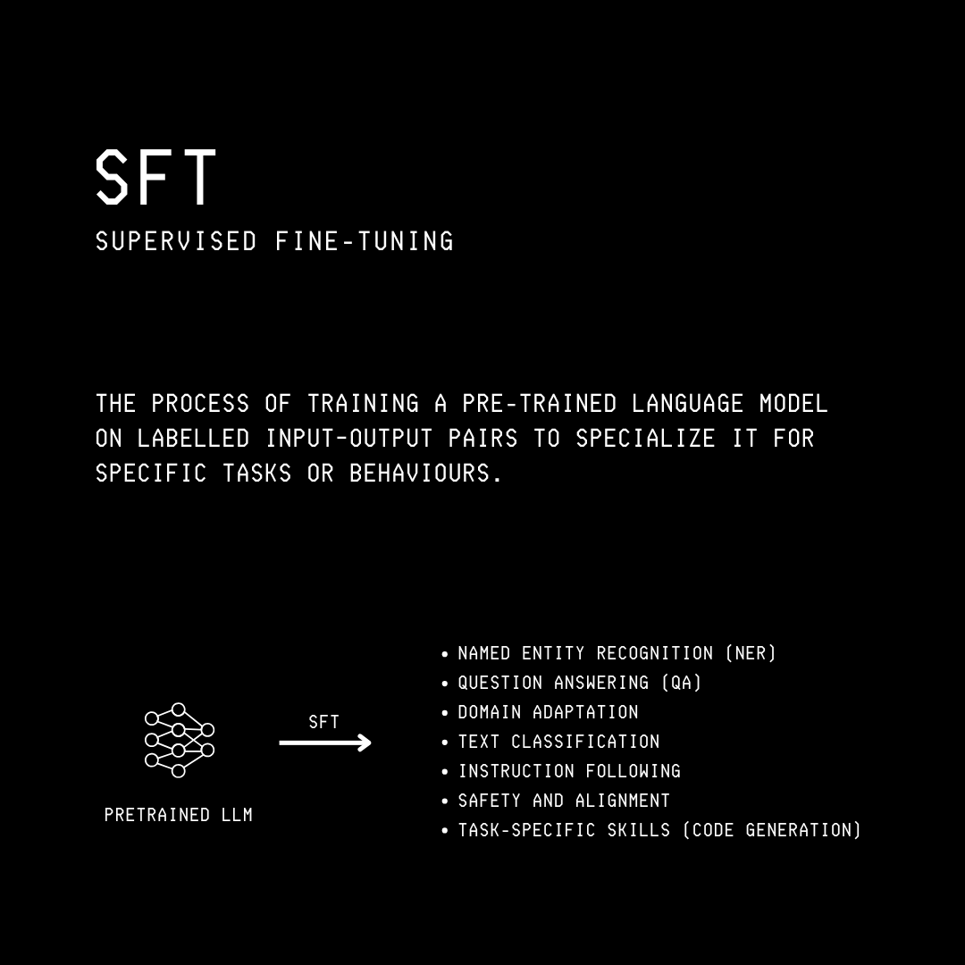
Training a model with SFT is followed by its RL training to align it with human values (using PPO) and to improve its reasoning (popularly using GRPO).

PPO vs. GRPO (Image from author’s book titled ‘LLMs In 100 Images’)

Previous research has shown that LLMs trained with SFT do not generalise well. This means that they can overfit to the training dataset and memorize it to a large extent.

This overfitting results from the large updates to the model parameters in each SFT step, especially when the distributions of the SFT training data and an LLM’s pre-training data differ.

Therefore, SFT-trained models may perform well in domain-specific tasks but tend to lose their general capabilities.

It has also been shown that SFT-trained models can lose their capability to explore and further improve with subsequent RL training.

This phenomenon is called Entropy collapse, where the LLM’s uncertainty in token selection (‘action’ in RL terms) rapidly decreases to near zero during training. This generates very predictable responses from the LLM rather than diverse ones.

To understand how SFT works better, let’s deep dive into the mathematics behind it.

---

The Mathematics Of Supervised Fine-Tuning

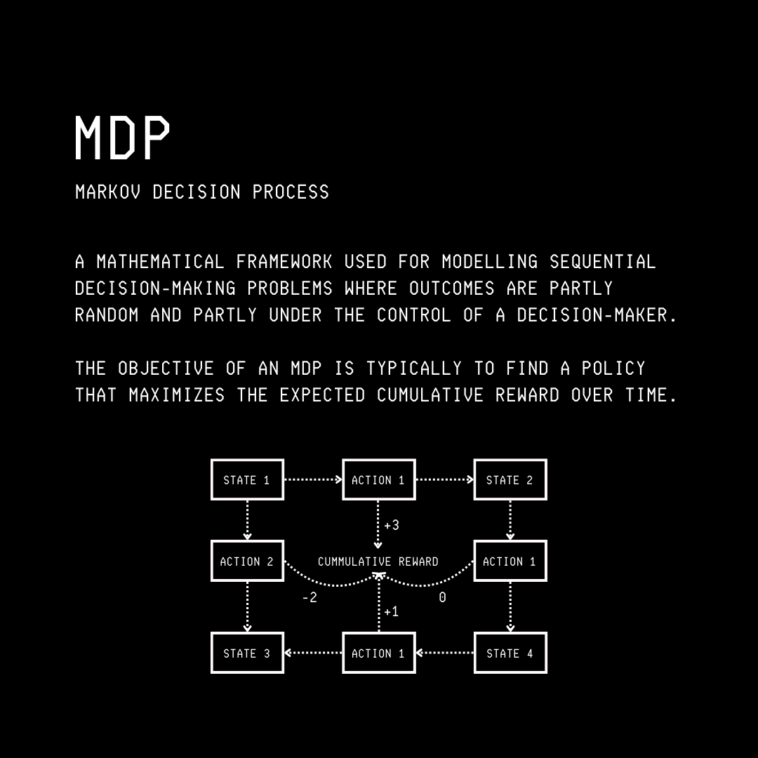
Let’s understand language modeling using a Markov Decision Process (MDP).

If you’re new to this term, Markov Decision Process, or MDP, is a mathematical framework that is used to model sequential decision-making problems and make optimal decisions when outcomes are uncertain.

In problems modeled by the MDP, the future state depends only on the current state and the chosen action, and not on the sequence of events that preceded it. This is called the Markov property.

Markov Decision Process (Image from author’s book titled ‘AI In 100 Images’)

An MDP is defined using:

• State space (S): A set of all possible states that an agent can be in.

• Action space (A): A set of all possible actions or moves the agent can take.

• Transition probability (P(s'|s, a)): The likelihood of moving from state s to s' when the agent takes an action a. It describes how the environment evolves when the agent takes an action in a given state.

For the MDP of autoregressive language modeling in LLMs:

• The state s(t) at timestep t is the current context, i.e., the input query x plus all tokens generated so far (y(<t)).
  All states, up to the final timestep (when the LLM stops generating tokens), form the state space.

• The action a(t) at timestep t is the next token y(t) chosen by the LLM.
  All actions (generated tokens) up to the final timestep are a part of the action space determined by an LLM’s vocabulary.

• When action a(t) is taken in the state s(t), the Transition probability is 1, since the chosen action/ token is simply added to the sequence, making the state evolve from (x, y < t​) to (x, y ≤ t​) in a deterministic way.

The LLM’s probability distribution over the following actions/ generated tokens is represented by π(θ)​ and called the Policy, which is stochastic in nature.

For a query x (with m tokens), the model generates an output y (with n tokens).

The joint probability of generating y given x is:

The joint probability of generating an output ‘y’ given query ‘x’ is the product of probabilities of each token ‘y(t)’ generated at each timestep ‘t’ given its preceding context (y(<t), x).

The training objective for SFT is to minimize the cross-entropy loss between the LLM’s predicted token distribution and the ground truth tokens.

It is mathematically represented using the following equation:

SFT loss per prompt-completion pair (x, y)

where:

• y(t) is the generated token at timestep t

• n is the total number of generated tokens

• y(<t), x is the context at each timestep

• π(θ)​ is the LLM with parameters θ called Policy in RL terms

Inspired by RL, for a training dataset D with multiple prompt-completion pairs, the SFT loss can be written as follows:

SFT loss minimized using gradient descent during training

where:

• s(t) is the context at time step t (‘state’ in RL terms)

• a*(t) represents the correct next token (correct ‘action’ in RL terms)

This loss is an expected value that averages the cross-entropy loss over all examples/ prompt-completion pairs in the training dataset D.

---

How Does SFT Relate To Reinforcement Learning?

Let’s learn a bit about some RL algorithms that come next in the post-training pipeline.

There are three main classes of RL algorithms for solving MDPs:

1. Value-based methods: These methods learn the value function and indirectly derive the policy using it. For example, Q-learning.

2. Policy gradient methods: These methods learn the policy directly without relying on a value function. For example, REINFORCE.

3. Hybrid methods: These combine both of the above. Examples include Actor-Critic (AC) algorithms such as TRPO and PPO.

AC algorithms have two components:

• An ‘Actor’ (the policy-based component) that determines which actions to take according to a policy function.

• A ‘Critic’ (the value-based component) that evaluates how good the actions are, according to a value function.

We will discuss specific AC algorithms in more detail soon. Let’s first understand Policy gradient methods in view of language modeling.

For a given LLM policy π(θ), we sample trajectories from it, or in simple words, record the sequences of states, actions, and rewards that it generates.

With RL training using Policy gradient, the LLM policy is optimized using the following objective:

Policy gradient objective maximized using gradient ascent during RL training

where:

• s(t), a(t) are state–action pairs sampled from the current policy π(θ)

• log π(θ)​(a(t)​|s(t)​) is the log-probability of the action the policy took

• Â(t) is the estimated advantage function at timestep t.
  This is a signal of how much better or worse an action a(t)​ was (given by the Q-function) compared to the policy’s average expectation at state s(t) (given by the Value function).

The advantage function is the difference between the Q function given an action taken in a particular state, and the Value function given a state.

If for an action, Â(t)​ > 0, this action is better than expected, and RL training increases its probability under the policy, and vice versa.

Can you notice how the Policy gradient objective is similar to the SFT loss?