RNNs Are Coming Back To Take Over Transformers (Yes, For Real!)
A deep dive into what RNNs, LSTMs, and GRUs are and how they are being modified to overcome the limitations of the currently prevalent Transformer architecture.
Transformers have transformed our world.
They are the dominant AI architecture for almost all sequential tasks today.
One reason the Transformer architecture did so well is its Self-attention mechanism, which allows the processing of tokens simultaneously rather than sequentially as in previous architectures such as RNN, LSTM, and GRU.
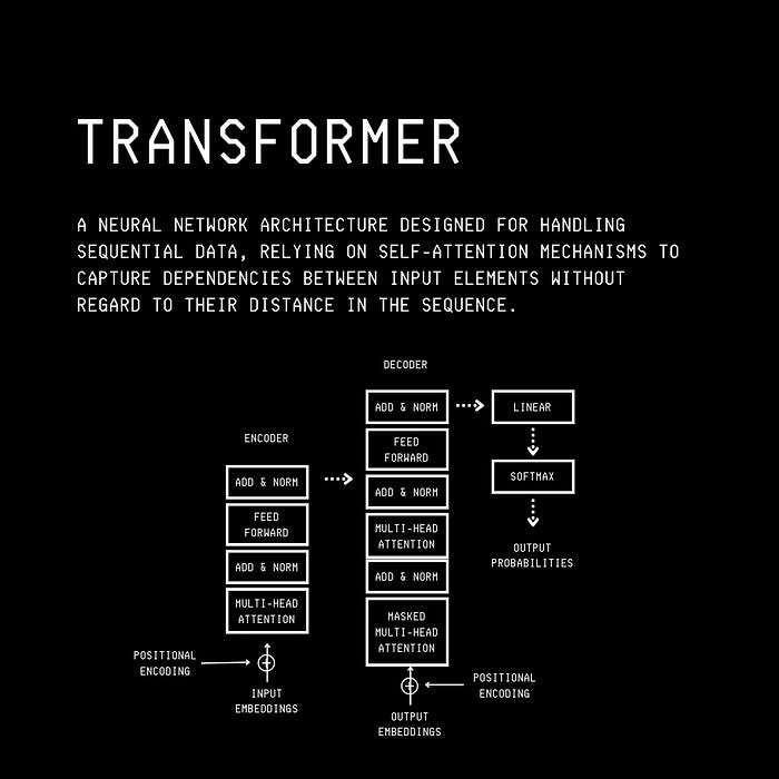
But Transformers are not perfect.
They have a quadratic computational complexity in the sequence length.
This means that as the length of the input sequence increases, the amount of computation required grows quadratically (square of the sequence length).
This is because of their Self-attention mechanism, where every token in the sequence pays attention to every other token to understand the context.
This limits Transformers significantly when processing long sequences in computationally resource-limited settings.
To fix this problem, researchers in a recent preprint of ArXiv have tweaked the internals of traditional LSTMs and GRUs, resulting in their minimal versions called minLSTMs and minGRUs.
These networks use far fewer parameters, can be trained in parallel, and are much faster than their traditional counterparts.
This is absolutely incredible!
Here is a story where we deep dive into what RNNs, LSTMs, and GRUs are and how they are being modified to overcome the limitations of the currently popular Transformer architecture.
Let’s go!
Why Did We Need RNNs In The First Place?
Multi-layer Perceptrons (MLPs) or Feed-forward Neural Networks cannot handle sequential data.
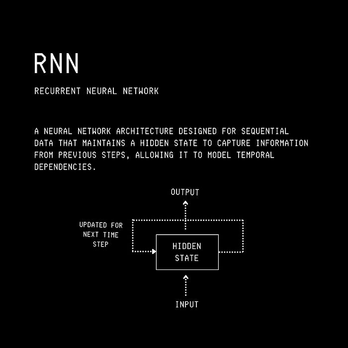
Hence, Recurrent Neural Networks (RNNs) were developed to solve this.
These neural networks use an internal hidden state or “memory” to process sequential information and maintain information about the previous inputs.
Using this memory, they can capture dependencies among different sequence elements separated by time steps (called Temporal dependencies).
RNNs are trained using Backpropagation Through Time (BPTT).
This is an extension of the standard Backpropagation algorithm used for Feed-forward neural networks.
BPTT involves unfolding the network over time and treating each time step like a layer in a Feed-forward neural network.
The Forward pass step processes the input sequence.
An error is calculated at the output layer, and the resulting gradients are backpropagated from the last time step to the first, updating the RNN’s parameters.

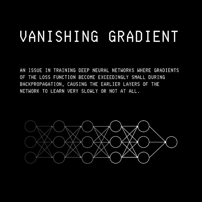
RNNs struggle with learning long temporal dependencies due to the Vanishing gradient problem.
This is when, during Backpropagation through time, gradients can become extremely small, leading to no learning.
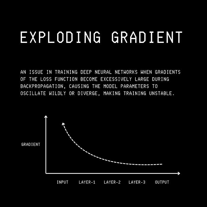
Things can go wrong the other way as well, with the gradients becoming too large, leading to unstable training.
This is called the Exploding gradient problem.
The LSTM (Long Short-term Memory) architecture was introduced to fix these challenges in 1997.
Let’s discuss it next.
The Birth Of LSTM
The LSTM architecture is a modification of the RNN that can retain long temporal information without suffering from the Vanishing / Exploding Gradient problems.
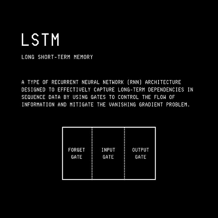
LSTM is composed of:
Cell state — to store long-term information
Hidden state — to carry the short-term output for the current time step
Three gates (Input, Forget, Output gates)
At each step, LSTM decides, based on multiple mathematical operations and gates, how much information to forget, how much to add to its cell state, and how much to output for the next step.
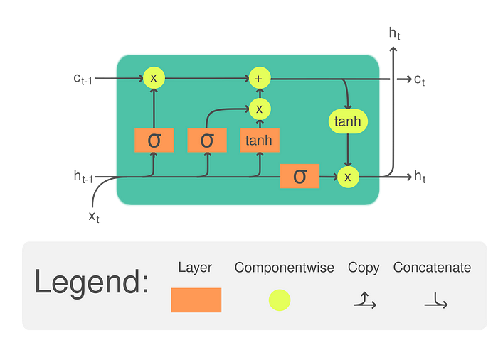
An LSTM module contains O(4d(h)(d(x) + d(h))) parameters, where d(h) is the size of the hidden state and d(x) is the size of the input vector x(t).
But could LSTM be further improved?
The Rise Of GRU
The Gate Recurrent Unit or GRU architecture was introduced in 2014, simplifying the LSTM.
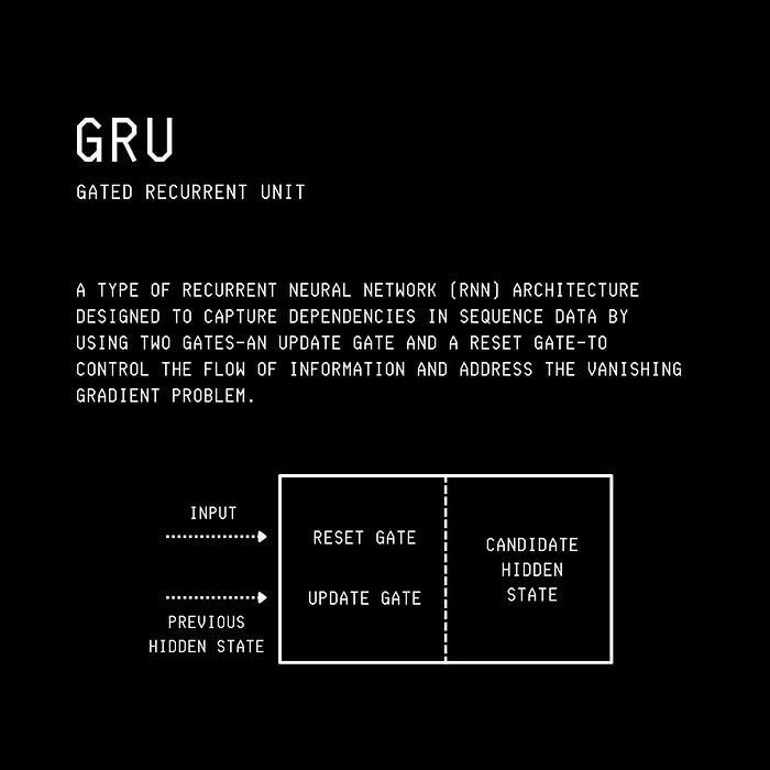
Instead of LSTM’s three gates and two states, it uses two gates and a single state.
In GRU, LSTM’s Forget and Input gates are combined into a single Update gate. This gate decides how much past information should be kept and how much of the new information should be added.
LSTM’s Output gate is replaced by a Reset gate in GRU. This gate determines how much of the past information should be “reset” or forgotten before adding new information.
These changes reduce the parameters of the network to O(3d(h)(d(x) + d(h))) , where d(h) is the size of the hidden state and d(x) is the size of the input vector x(t).
This leads to faster training and inference times than LSTM.
Both LSTM and GRU are trained sequentially using Backpropagation through time (BPTT).
This requires linear training time, which limits their ability to scale to long input sequence lengths.
The Rule Of Transformers
In 2017, Transformers took over the sequential processing task domain completely.
Their Self-attention mechanism allows every token in the sequence to pay attention to every other token simultaneously (rather than sequentially) to understand the context.
This approach makes the architecture parallelizable.
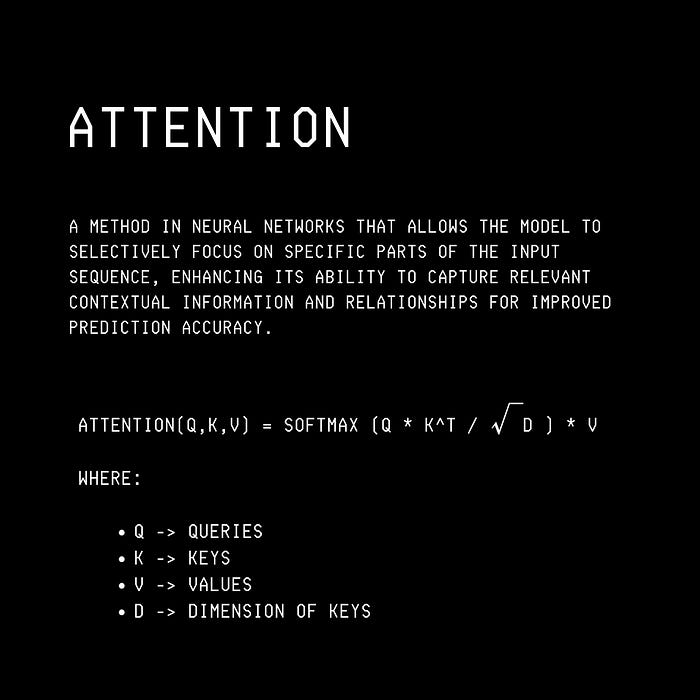
Self-attention has its advantages, but it introduces quadratic time complexity in sequence length, limiting the Transformer’s capability to scale to long contexts.
What if we could find models that fix this limitation of Transformers?
The Answer Lies in RNNs Itself
Researchers show that LSTMs and GRUs can be simplified by removing many hidden state dependencies from their different gates (and making a few other changes, which are discussed in the next section).
This can remove the dependency of these architectures to be trained using Backpropagation Through Time (BPTT).
If not BPTT, then what?
An algorithm called the Parallel Prefix Scan algorithm can be used to train these modified versions of LSTM and GRU.
This algorithm efficiently computes prefix operations over a sequence of data points using an associative operator (e.g., addition or multiplication).
By breaking a problem into smaller pieces, the algorithm allows for solving them in parallel.
Mathematically, the algorithm can be described as follows —
where ⨁ is an associative binary operator (i.e. addition or multiplication) applied to elements u(i) and positions k.
The algorithm computes the result y(k) in parallel with a time complexity of O(log(N)) instead of sequentially, which would take O(N) time on N processors.
This can be used to solve the following kind of equation in parallel.

Interestingly, this equation is a part of the LSTM and GRU architecture.
Let’s discuss how, next.
Simplifying GRU Towards ‘minGRU’
In minGRU, the dependencies of the update gate and the candidate hidden state on the previous hidden state are removed.
This allows the application of the Parallel Prefix Scan algorithm on the resulting equation.
Additionally, in a GRU, the tanh (Hyperbolic tangent) activation function is used to constrain the values of the candidate hidden state to the range (-1, 1).
This restriction stabilises the training by preventing the hidden states from becoming too large and avoiding the Vanishing gradient problem.
In minGRU, this tanh activation is removed, resulting in simpler and faster training.
Both of these changes are shown below.

Resultantly, minGRU requires only O(2 * d(h) * d(x)) parameters in comparison to GRU’s O(3 * d(h) (d(x) + d(h))) where d(h) and d(x) represent the sizes of the input and hidden state, respectively.
Along with this, it can now be trained in parallel.
Simplifying LSTM Towards ‘minLSTM’
In minLSTM, the dependencies of the cell state, forget gate and the input gate are removed from the previous state.
This makes its equations parallelizable using the Parallel Prefix Scan algorithm.
Similar to minGRU, the tanh activation function is removed from the calculations of the cell state and the hidden state.
There is one last change in the LSTM architecture that turns it into minLSTM.
In traditional LSTMs, the Input and Forget gates are computed independently. Hence there’s no guarantee that their combined effect on the combined effect will remain stable across time steps.
This introduces time-dependent scaling i.e. the scale of the hidden state can vary with time.
To fix this, the Forget gate and the Input gate are normalized to ensure that their sum is always equal to 1.
To ensure that the hidden state is time-independent in scale, the output gate and the hidden state are directly linked to the cell state.
This also drops the original cell state, as the hidden state takes over its role.
Note that GRUs do not need this step as their outputs are already time-independent in scale.
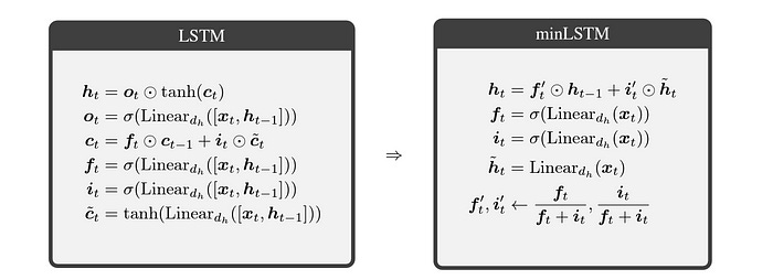
Resultantly, minLSTM requires only O(3 * d(h) * d(x)) parameters in comparison to LSTM’s O(4 * d(h) (d(x) + d(h))) where d(h) and d(x) represent the sizes of the input and hidden state, respectively.
Alongside, it can now be trained in parallel.
How Well Do These RNNs Perform?
Runtime Performance
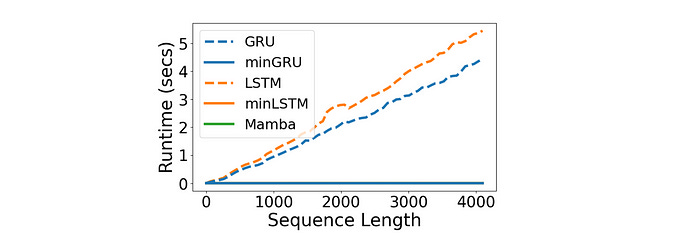
The runtime for minLSTM and minGRU is significantly faster than that of their traditional counterparts.
Notably, minGRUs and minLSTMs are 1324× and 1361× faster for a sequence length of 4096, respectively, compared to GRUs and LSTMs.
In layman's terms, where minGRU would take a day to finish training, its traditional counterpart GRU could take over three years!
Compared with Mamba, a state space model, both minLSTM and minGRU have similar runtime performance.
Memory Use
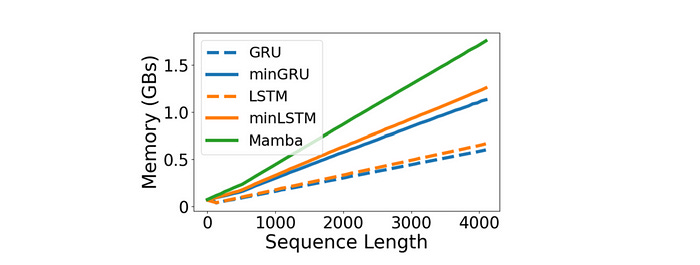
minGRU and minLSTM require 88% more memory compared to their traditional counterparts.
This is because they use the parallel prefix scan algorithm, leading to larger computational graphs.
The same is true for Mamba, which requires around 56% more memory than minGRU.
This is not worrying because, during training, the bottleneck for RNNs is typically the runtime.
Speedup
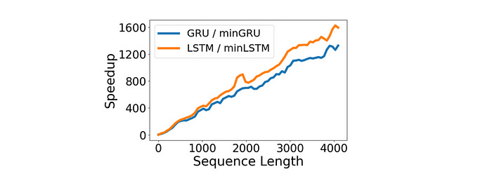
Requiring fewer parameters, the minLSTM model achieves a 235× speedup, and the minGRU model achieves a 175× speedup in training for a sequence length of 512 on a T4 GPU compared to their traditional counterparts.
Training Stability
minGRU is more stable than minLSTM during training.
The reason is that minGRU has a single set of parameters (i.e., the Update gate) to update, as compared to minLSTM, which has two sets of parameters (i.e., the Forget and Input gates).
This makes minGRUs easier to optimize.
Performance in Reinforcement Learning
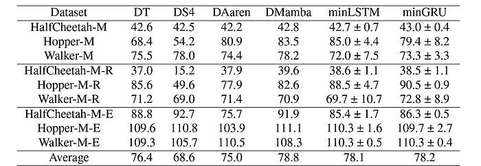
These architectures perform quite well when evaluated on the MuJoCo (Multi-Joint dynamics with Contact) locomotion tasks from the D4RL benchmark.
They are better than Decision S4 and perform competitively with Aaren, Decision Mamba, and Decision Transformer architectures.
Performance in Language Modelling
For this evaluation, a character-level GPT was trained on Shakespeare's works based on the NanoGPT framework by Andrej Karpathy.
minLSTM and minGRU perform remarkably well here.
Both, along with Mamba and Transformers, achieved similar test losses.
It should be noted that minGRU, minLSTM, Mamba and Transformers have comparable test losses of 1.548, 1.555, 1.575 and 1.547. respectively.
Additionally, minGRU and minLSTM trained 2.5x faster than Transformers to reach comparable performance.
This is because of their linear time complexity with sequence length compared to Transformer’s quadratic complexity.

These surprising findings make us question if “Were RNNs all we needed?”.
I am excited about the advancements that will come after reintroducing these highly efficient RNNs.
What are your thoughts on them? Let me know in the comments below.


