ML Interview Essentials: Building Self-Attention From Scratch

#1. Self-Attention (7 minutes read)

Nov 02, 2025

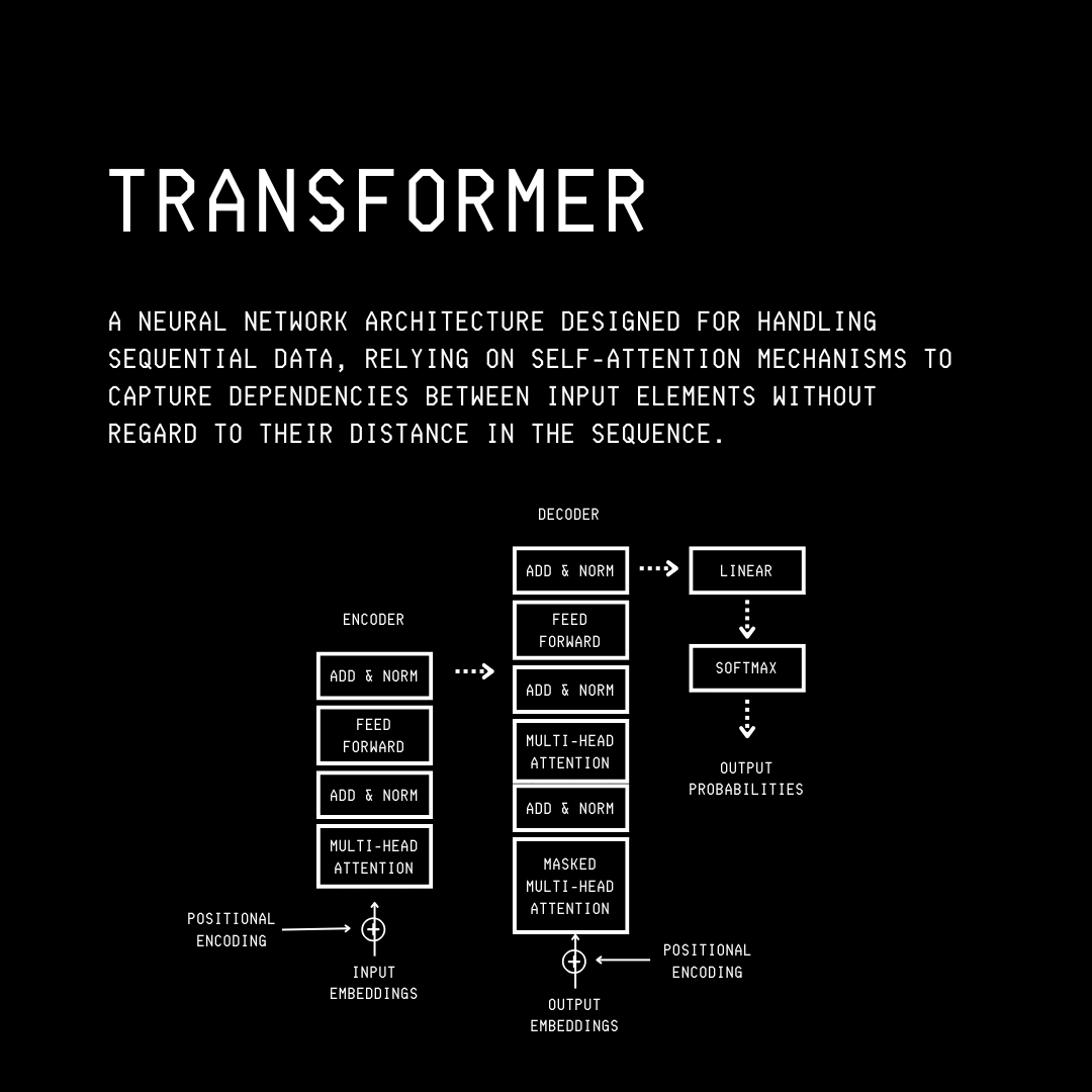
The Transformer is the backbone of all popular LLMs that we use today.

The original Transformer architecture, developed by Google researchers in 2017, consists of encoder and decoder blocks and was primarily designed for language translation.

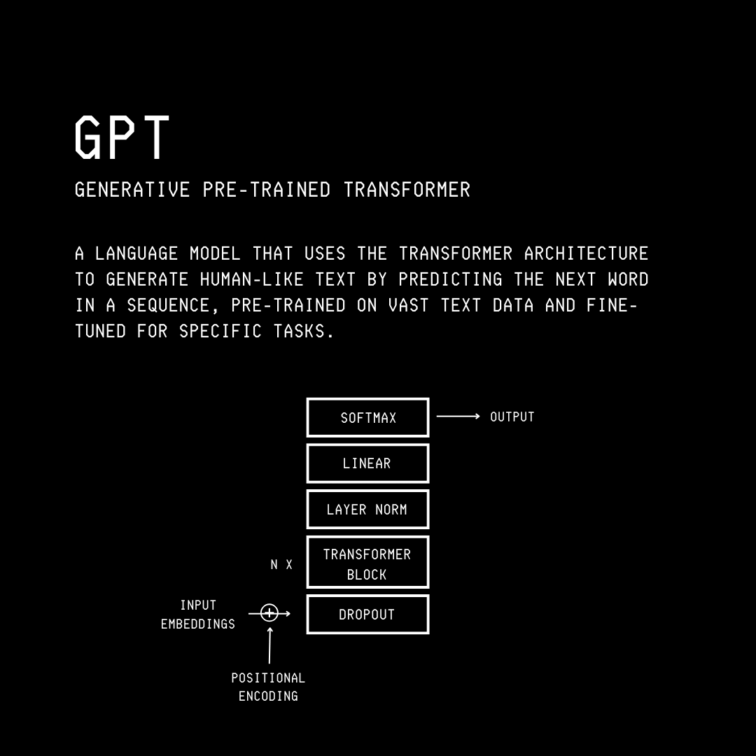
Transformer visualised (Image from author’s book titled ‘**LLMs In 100 Images**')

This architecture was modified into the Decoder-Only Transformer, leading to the Generative Pre-trained Transformer (GPT) by OpenAI in 2018.

Primarily designed for text generation, it is widely used by today's LLMs.

GPT visualised (Image from author’s book ‘**LLMs In 100 Images**’)

What makes this architecture so powerful is that, unlike previous methods (RNNs), it allows LLMs to understand and process all words in the input text in parallel, rather than one after another (sequentially).

This is achieved through a mechanism called Self-attention, which helps determine how each word relates to every other word in the same text sequence.

(Note that this is different from Cross-attention, which computes relationships between two different input sequences, so that they can attend to each other.)

Let’s learn how to code up Self-attention from scratch in this tutorial.

We Begin With Text Pre-Processing

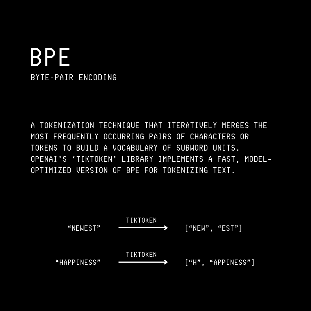
Any sentence given to an LLM must first be broken down into small pieces called Tokens in a process called Tokenization. In LLMs like GPT, this is done using a Tokenization algorithm called Byte Pair Encoding.

BPE visualised (Image from author’s book titled ‘**LLMs In 100 Images**’)

The resulting tokens are then encoded into Token Embeddings, which are high-dimensional vector representations of the tokens.

Since the Transformer architecture processes tokens in parallel, it has no way of knowing the order of tokens in a given sentence. Positional Encodings are therefore used to represent the positional information of tokens.

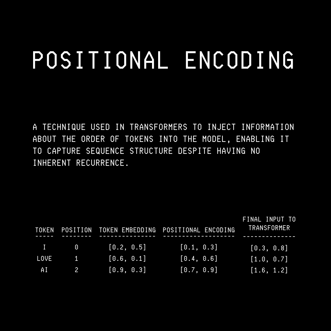
Positional Encodings visualised (Image from author’s book titled ‘**LLMs In 100 Images**‘)

These are combined with the input token embeddings to create the final token embedding representation, which is then passed to the Self-attention mechanism.

Building Self-Attention

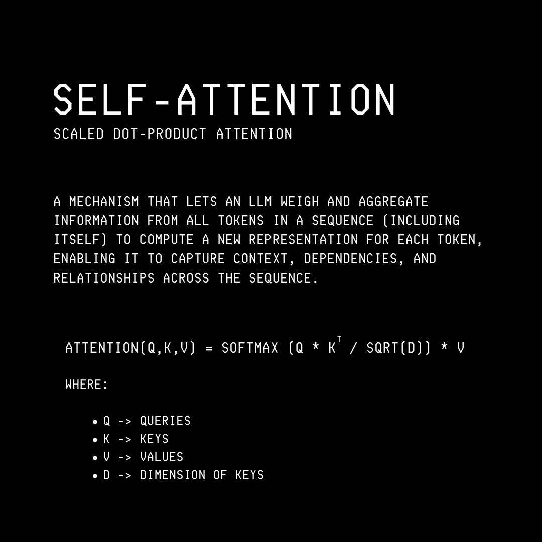
The Self-attention mechanism is also called Scaled Dot-product Attention, and this is what we will be building in this tutorial.

Self-attention visualised (Image from author’s book titled ‘**LLMs In 100 Images**’)

Let’s assume that we have:

A batch of two sentences (batch_size)
Each with six tokens (sequence length), and
Each token embedding is of dimension 4 (embedding_dim)

The resulting input embedding is as follows:

import torch 

batch_size = 2
sequence_length = 6
embedding_dim = 4

# Create embeddings for a batch
input_embeddings = torch.rand(batch_size, sequence_length, embedding_dim)

print(input_embeddings)

tensor([[[0.6396, 0.0421, 0.3705, 0.3118],
         [0.9372, 0.9827, 0.5099, 0.1424],
         [0.6218, 0.5806, 0.4458, 0.9932],
         [0.1567, 0.3385, 0.4156, 0.1641],
         [0.0769, 0.1863, 0.6174, 0.4750],
         [0.6468, 0.3951, 0.7799, 0.8695]],

        [[0.5449, 0.7488, 0.7040, 0.4991],
         [0.1247, 0.0083, 0.8410, 0.7563],
         [0.3166, 0.6144, 0.0426, 0.4958],
         [0.8346, 0.9443, 0.8406, 0.9150],
         [0.7565, 0.1786, 0.6084, 0.6638],
         [0.9564, 0.3453, 0.3544, 0.3614]]])

The shape of this embedding is [2, 6, 4] ([batch_size, sequence_length, embedding_dim]).

Creating Queries, Keys, and Values

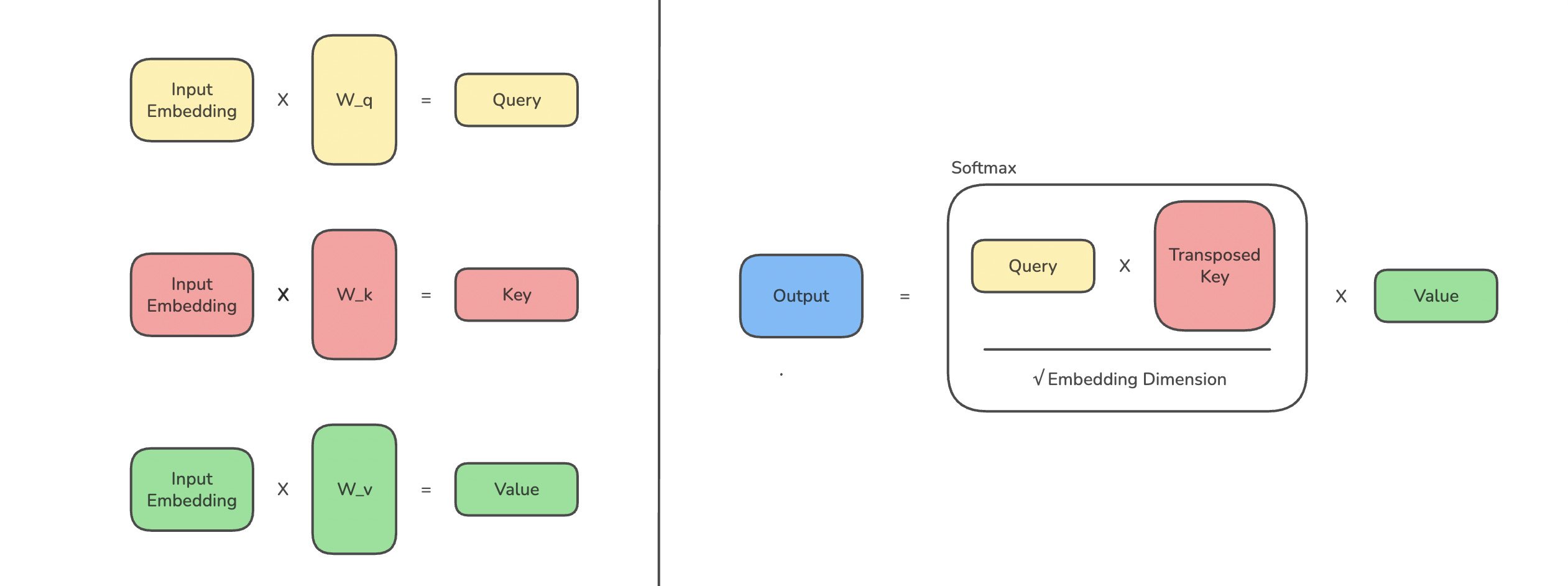
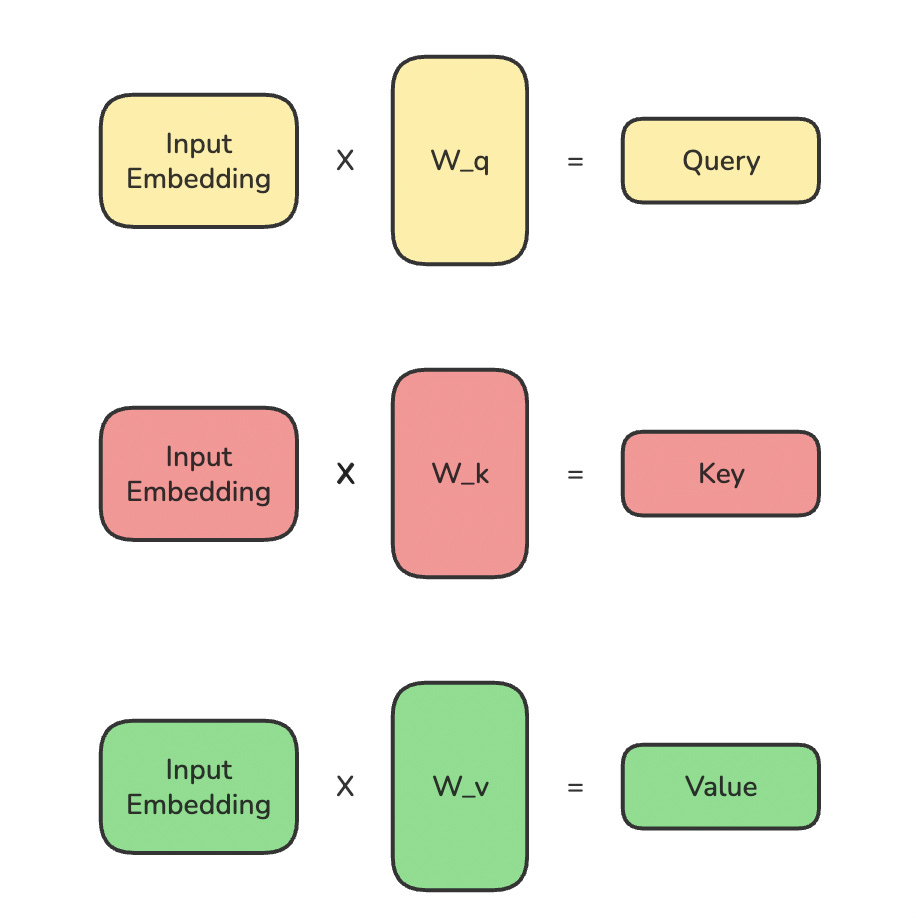
This embedding is converted into Queries (Q), Keys (K), and Values (V) using three matrices W(Q), W(K), and W(V), respectively.

# Create learnable projection matrices (weights)

W_q = torch.rand(embedding_dim, embedding_dim, requires_grad=True)
W_k = torch.rand(embedding_dim, embedding_dim, requires_grad=True)
W_v = torch.rand(embedding_dim, embedding_dim, requires_grad=True)

# Project input embeddings to Q, K, V

Q = input_embeddings @ W_q  
K = input_embeddings @ W_k  
V = input_embeddings @ W_v

This is how the operation looks.

Calculating Attention Scores & Attention Weights

From here, we calculate the attention scores by multiplying the Queries by the Keys.

# Calculate Attention scores

attn_scores = Q @ K.transpose(-2, -1)

Next, we scale the scores and apply softmax to get attention weights.

Scaling by the square root of the embedding dimension prevents dot-product attention scores from growing too large as the embedding dimension increases. Without this scaling, large dot products would push the softmax into regions with extremely small gradients, causing training instability.

# Calculate Attention weights

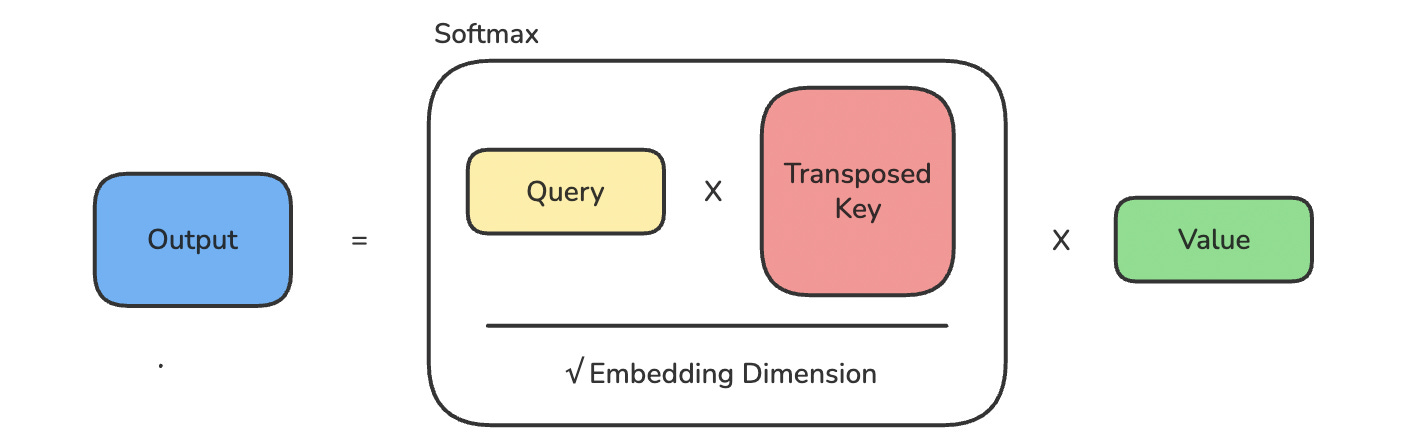
attn_weights = torch.softmax(attn_scores / embedding_dim**0.5, dim=-1)

Finally, the attention weights are multiplied by the Values to create the output.

# Create output

output = attn_weights @ V

These operations are shown together in the image below.

Self-Attention At Work

Let’s pack everything into a reusable SelfAttention class.

import torch
import torch.nn as nn

class SelfAttention(nn.Module):
    def __init__(self, embedding_dim):
        super().__init__()
        self.embedding_dim = embedding_dim
        
        # Learnable projection matrices for Q, K, V
        self.W_q = nn.Linear(embedding_dim, embedding_dim, bias=False)
        self.W_k = nn.Linear(embedding_dim, embedding_dim, bias=False)
        self.W_v = nn.Linear(embedding_dim, embedding_dim, bias=False)
    
    def forward(self, x):
        # Project input to Q, K, V
        Q = self.W_q(x)  
        K = self.W_k(x)  
        V = self.W_v(x) 
        
        # Calculate Attention scores
        attn_scores = Q @ K.transpose(-2, -1) 
        
        # Scale and apply softmax to get Attention weights
        attn_weights = torch.softmax(attn_scores / self.embedding_dim**0.5, dim=-1)
        
        # Multiply Attention weights by values (V)
        output = attn_weights @ V  
        
        return output, attn_weights

We use nn.Linear in the SelfAttention class, instead of torch.rand because it automatically manages weights, gradients, and initialization.

Let’s pass our input embedding through this attention mechanism.

# Initialize Self-attention layer
self_attn = SelfAttention(embedding_dim)

# Forward pass 
output, attn_weights = self_attn(input_embeddings)

tensor([[[ 0.1632,  0.0137,  0.0873,  0.4781],
         [ 0.1617,  0.0126,  0.0861,  0.4769],
         [ 0.1611,  0.0120,  0.0856,  0.4765],
         [ 0.1614,  0.0121,  0.0857,  0.4770],
         [ 0.1628,  0.0141,  0.0875,  0.4760],
         [ 0.1613,  0.0125,  0.0861,  0.4748]],

        [[ 0.1381, -0.1087,  0.0680,  0.4477],
         [ 0.1374, -0.1087,  0.0674,  0.4479],
         [ 0.1388, -0.1066,  0.0689,  0.4477],
         [ 0.1370, -0.1107,  0.0669,  0.4479],
         [ 0.1385, -0.1071,  0.0685,  0.4478],
         [ 0.1373, -0.1085,  0.0673,  0.4481]]], grad_fn=<UnsafeViewBackward0>)

Note that the Self-attention mechanism preserves the shape of the input ([batch_size, seq_len, embedding_dim]). This lets us stack multiple Self-attention layers together in a Transformer block.

print(”Input shape:”, input_embeddings.shape)
print(”Output shape:”, output.shape)

Input shape: torch.Size([2, 6, 4])
Output shape: torch.Size([2, 6, 4])

Complexity of Self-Attention

Where n = sequence_length and d = embedding_dim

Time Complexity: The time complexity of Self-attention is O(n²d) because we compute attention scores between every pair of tokens (n²), and each score requires a dot product of d-dimensional vectors.
Space Complexity: The space complexity is O(n² + nd) because we need O(n²) space to store the attention score matrix (n × n) and O(nd) space to store the Q, K, and V matrices (each n × d).

That’s everything for the Self-attention mechanism. See you soon in the next lesson, where we extend this to Multi-head attention.

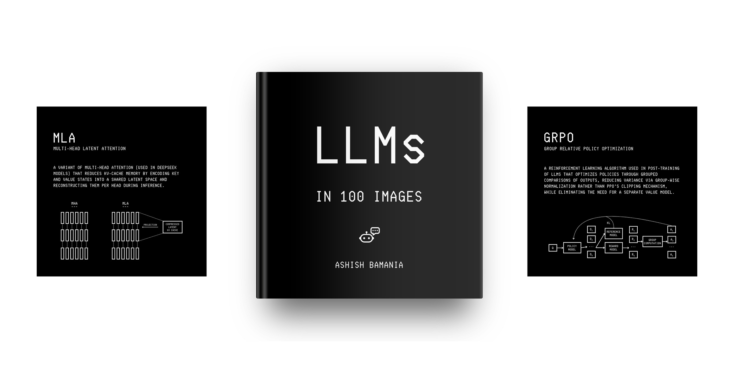
Images used in this article are taken from my book ‘LLMs In 100 Images’.

It is a collection of 100 easy-to-follow visuals that explain the most important concepts you need to master to understand LLMs today.

Grab your copy today at a special early bird discount using this link.