

A Detailed History of Optimizers (And How The New ‘Adam-mini’ Optimizer Works)
A deep dive into how Optimizers work, the history of their development, and how the novel 'Adam-mini' optimizer enhances LLM training like never before


An Optimizer forms the basis for training most modern neural networks.
Published in 2017, the Adam Optimizer, along with its variants, has become the dominant and go-to optimizer for training LLMs in the industry today.
But there’s an issue with Adam that has been largely overlooked due to its superior performance.
That issue is Memory inefficiency.
To train an LLM with 7 billion parameters, Adam requires around 86 GB of memory.
For models like Google PaLM, which consists of 540 billion parameters, more than 50 GPUs are needed just to contain Adam itself.
But maybe not anymore. Here’s some exciting news!
A team of ML researchers have developed a better version of Adam called Adam-mini.
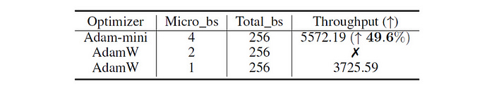
The Adam-mini optimizer is twice as memory efficient and achieves 49.6% higher throughput than AdamW when used to train billion-parameter LLMs.
This is a story where we deep dive into how Optimizers work, how they were developed, what their limitations are, and how Adam-mini solves some of these to serve as a breakthrough for the future of deep learning.
But First, What Are Optimizers?
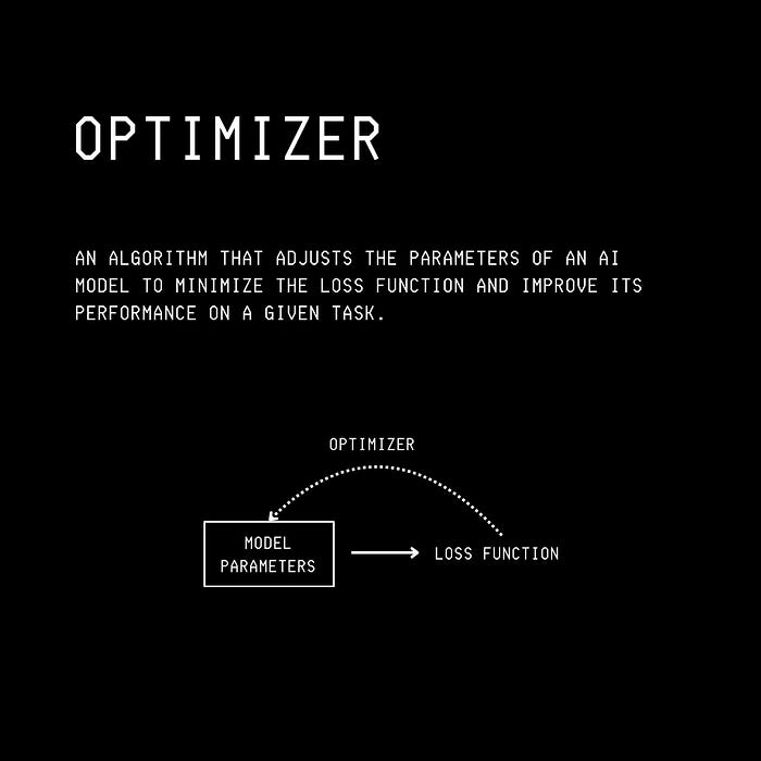
An Optimizer is an algorithm that adjusts an ML model's parameters (weights and biases) to minimize the Loss function.
This leads to a more accurate model during model training.
We must start with the most basic optimization algorithm, called Gradient Descent, to understand how modern Optimizers work.
Let’s learn about it.
What Is Gradient Descent?
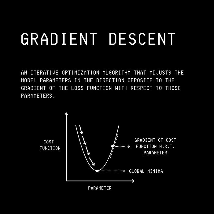
Gradient Descent is the foundational mathematical optimization algorithm that aims to minimize a loss function for an ML model iteratively.
During model training, it starts with an initial set of parameters and calculates the gradient of the loss function for each parameter.
(For those new to this term, the gradient is a vector of the first-order partial derivatives of the loss function with respect to the model parameters.
The loss function's gradient indicates its direction and rate of change with respect to each parameter.)
Next, using these gradient calculations, the optimizer iteratively updates the model’s parameters in the opposite direction to the gradient to reduce the loss function.
This can be thought of as following the direction of the slope of the surface of a mountain (here, created by the loss function) downhill until we reach a valley.
The algorithm can be mathematically expressed as —

θ is a model parameter, α is the learning rate that controls the step size during Gradient Descent, and∇L(θ) is the gradient of the loss function with respect to the parameter θ (Image created by author)Variants of Gradient Descent
The Gradient Descent algorithm has three variants based on how the loss function’s gradient is calculated.
Batch Gradient Descent (BGD)
In this variant, the entire dataset is used to compute the gradient of the loss function with respect to the parameters to perform just one update of the model parameters.

m’ is the number of training data points and ∇L(i)(θ) is the gradient of the loss function with respect to the parameter θ for the i-th data point (Image created by author)This approach leads to stable convergence but can be very slow and memory-inefficient for large datasets.
2. Stochastic Gradient Descent (SGD)
In this variant, the gradient is computed using one training data point at a time for one update of the model parameters.

∇L(i)(θ) is the gradient of the loss function with respect to the parameter θ for the i-th data point (Image created by author)This approach is fast but leads to noise when the gradients are updated.
3. Mini-Batch Gradient Descent (MBGD)
In this variant, a subset of the training dataset (mini-batch) is used to compute the gradient of the loss function with respect to the parameters to perform one update of the model parameters.

B’ is a mini-batch of training data points and ∇L(i)(θ) is the gradient of the loss function with respect to the parameter θ for the i-th data point (Image created by author)This approach offers a good balance between the deficiencies in Batch Gradient Descent and Stochastic Gradient Descent.
However, it still has many shortcomings, which leads to sub-optimal convergence.
Here are a few major ones —
The same learning rate is applied to all parameter updates
The learning rate is fixed and does not adapt to the training dataset’s features
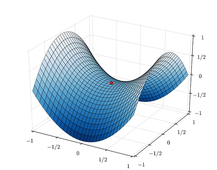
For non-convex loss functions, the algorithm can get trapped in local minima and on saddle points (shown in the image below)
Modern Optimizers To The Rescue
Most modern optimizers build upon the deficiencies of Gradient Descent and its variants.
(It must also be noted that many other optimization techniques, such as Particle Swarm Optimization and Bayesian Optimization, exist but do not rely on Gradient Descent.)
Let’s learn about some intermediate optimizers that lead to Adam and its variants (AdamW).
Momentum
Momentum builds on the shortcoming of Stochastic Gradient Descent (SGD), which is that it tends to get stuck in local minima.
The idea behind it is to build inertia using a velocity term that accumulates past gradients and helps maintain a consistent direction during parameter updates.

θ(t) and θ(t+1) is the parameter at iterations t and t+1 , respectively, v(t) is the velocity at iteration t , β is called the momentum factor, η is the learning rate and ∇θL(θ(t)) is the gradient of the loss function with respect to the parameter θ at iteration t (Image created by author)AdaGrad (Adaptive Gradient)
AdaGrad fixes the shortcoming of Stochastic Gradient Descent (SGD), which is that it uses a fixed learning rate for all parameters of the ML model.
Instead, AdaGrad adjusts the learning rate based on the parameters, making larger updates on infrequent parameters and smaller updates on frequent ones.
This is done by accumulating the squared gradients for each parameter and using this value to scale the learning rate.

θ(t) and θ(t+1) is the parameter at iterations t and t+1 , respectively, G(t) is the accumulated sum of the squares of the past gradients, η is the learning rate, ϵ is a small constant that prevents zero division error, and ∇θL(θ(t)) is the gradient of the loss function with respect to the parameter θ at iteration t (Image created by author)RMSProp (Root Mean Square Propagation)
RMSProp, like AdaGrad, adapts to the learning rate for each parameter based on past gradients.
But, since AdaGrad does this by keeping track of all past squared gradients, it leads to a continuously decreasing learning rate.
RMSProp solves this by using an exponentially decaying average of past squared gradients, leading to a consistent learning rate.

θ(t) and θ(t+1) is the parameter at iterations t and t+1 , respectively, η is the learning rate, β is the decay rate for the moving average of squared gradients, E[g²](t-1) is the exponentially decaying average of past squared gradients up to iteration t-1, ϵ is a small constant that prevents zero division error, and ∇θL(θ(t)) is the gradient of the loss function with respect to the parameter θ at iteration t (Image created by author)But could a better optimizer be created?
Here Comes ‘Adam’ (Adaptive Moment Estimation)
Adam, published in 2017, has become the backbone of training most neural networks today.
It combines the qualities of Momentum and RMSProp by tracking the gradients' first and second-moment estimates.
First Moment Estimate (Mean of the gradients)
Similar to Momentum, it keeps track of an exponentially decaying average of past gradients.

2. Second Moment Estimate (Uncentered Variance of the gradients)
Similar to RMSProp, it maintains an exponentially decaying average of previous squared gradients.

These terms are bias-corrected, leading to the following update rule for Adam.

θ(t) and θ(t+1) is the parameter at iterations t and t+1 , respectively, η is the learning rate, m^t and v^t are bias-corrected first and second-moment estimates, respectively, and ϵ is a small constant that prevents zero division error (Image created by author)Taking ‘Adam’ A Step Ahead With ‘AdamW’
Adam was further improved when an approach called AdamW was proposed in 2019.
AdamW decouples the Weight decay (L2 regularization) term from the gradient update process.
The Weight decay term (ηλθ(t)) is rather added directly to Adam's parameter update rule.

This helps AdamW attain better generalization performance than the standard Adam optimizer.
AdamW is widely adopted in the industry today, and Meta’s Llama family of LLMs have been notably trained using this optimizer.
But Wait, There's More. It's Time For ‘Adam-mini’!
AdamW isn’t perfect.
It is highly memory intensive.
It requires a lot of memory to store the first-order and second-order moment estimates, which is at least twice the memory of the model size.
To make this work, CPU offloading (transferring the computational workload from the GPU to the CPU) and Sharding (distributing the computation workload across multiple GPUs) have been used.
Unfortunately, these increase the latency and, in turn, slow down model training.
Hence, a new approach to modify AdamW was proposed.
AdamW assigns an individual learning rate to each parameter based on the gradient moment estimates in its current implementation.
This means that if we have a billion-parameter model, AdamW will allocate a billion different learning rates.

The researchers questioned this notion, asking —
“Is it really necessary to use an individual learning rate for each parameter?”
The answer to this was found to be — No.
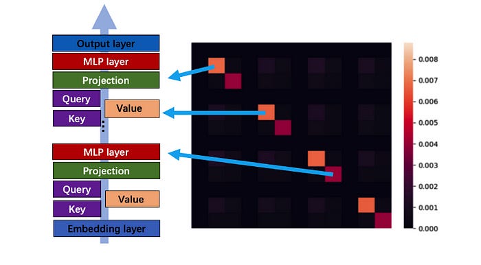
They noticed that the Hessian Matrix of a Transformer has a near-block diagonal structure, where diagonal elements are significantly larger than the off-diagonal elements.
(For those new to this term, a Hessian Matrix is a matrix consisting of the second-order partial derivates of the loss function with respect to the model parameters. It captures the loss function’s curvature and helps optimise model training.)
These dense sub-blocks are of different sizes and consist of groups of closely related parameters.
Specifically, the different components of the Transformer architecture — namely, the Query, Key, Value, and MLP layers — form these smallest distinct sub-blocks.
This insight led the researchers to develop Adam-mini.
In this algorithm, the model parameters are first partitioned into blocks based on the Transformer’s Hessian structure.
The Query and Key parameters are partitioned by heads, and the default PyTorch partition is used for all other parameters.
Next, a single learning rate is chosen for all of the parameters in each block, calculated by averaging the second moment estimates within that block.
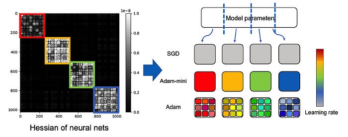
For example, for a model with five parameters, AdamW assigns each parameter its own learning rate based on the second moment estimate as follows.

In Adam-mini, on the contrary, parameters within each block are assigned a single learning rate by averaging the second moment estimates within that block, which greatly reduces the total number of learning rates used.

The detailed second-moment estimate calculation is shown below.

The Performance of ‘Adam-mini’
The overall performance of Adam-mini is quite exceptional, as demonstrated by various indicators.
Memory Efficiency
Adam-mini can reduce more than 90% of the second-moment estimates (denoted by v) used by different LLMs.
This saves up to 45% to 50% memory compared to AdamW.

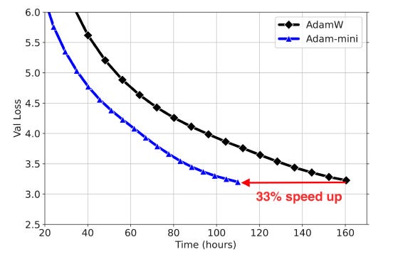
Throughput
Adam-mini largely reduces the communication among CPUs and GPUs due to its memory efficiency.
Also, Adam-mini’s update rules do not introduce any extra computations. All they do is average the second-moment estimates, which is a computationally cheap operation.
These lead Adam-mini to achieve a 50% higher throughput than AdamW, reducing 33% wall-clock time for pre-training Llama2–7B.
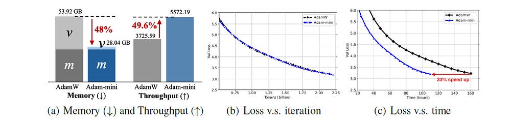
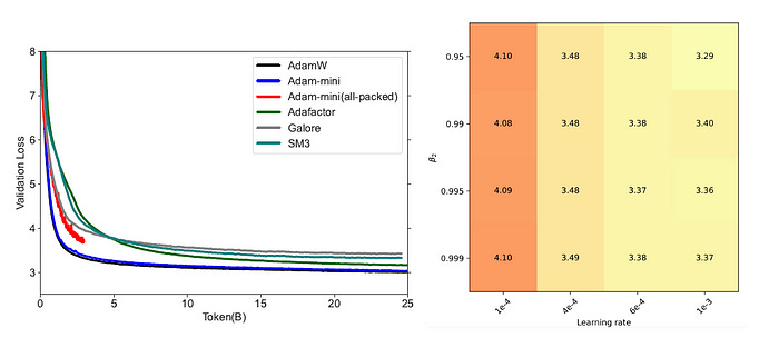
Performance On LLM Pre-Training
On Pre-training open-source LLMs from the Llama and GPT-2 series from scratch, Adam-mini matches the performance of AdamW while utilizing less memory.
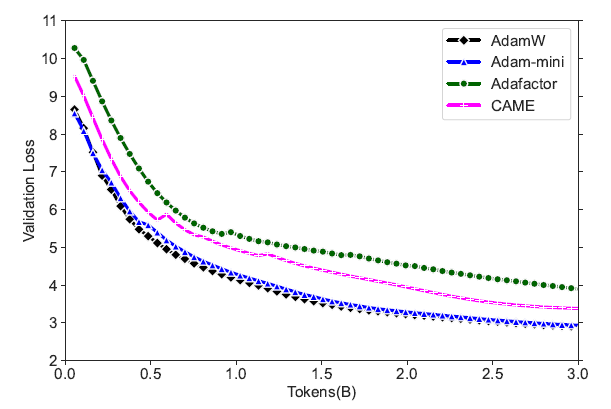
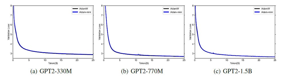
It is also noted that Adam-mini is not sensitive to hyperparameters and maintains a stable validation loss during training.
Performance on LLM Supervised Fine-Tuning
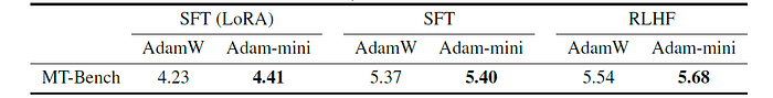
Supervised fine-tuning (SFT) of the Pre-trained Llama-2–7b model with and without LoRA (Low-Rank Adaptation) shows that Adam-mini performs better in terms of smaller evaluation Perplexity with less memory usage.
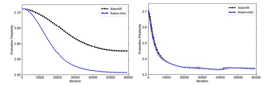
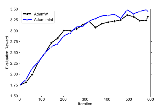
Similar findings regarding higher Evaluation rewards are noted when Reinforcement Learning from Human Feedback (RLHF) is implemented on the same LLM.
Next, as evaluated on the MT-Bench benchmark, the model's fine-tuning performance in terms of its chat ability shows that Adam-mini outperforms AdamW in each downstream task.
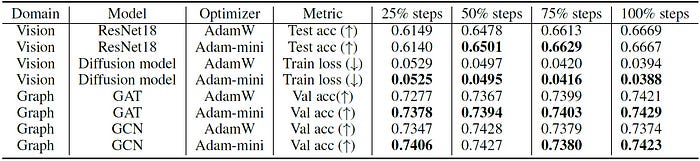
Performance on Non-LLM Tasks
The researchers also devised a version of Adam-mini for non-LLM neural networks.
The algorithm first groups parameters into blocks, by layers or other logical divisions within the model.
The second-moment estimates within each block of parameters are then averaged, and based on this, each block of parameters is assigned a single learning rate.
It is noted that Adam-mini performs at par or better than AdamW on all popular Non-LLM tasks.
These results are groundbreaking!
They will enable future researchers to train LLMs (and other deep neural network architectures) with fewer GPUs, reducing costs and energy use, further accelerating ML research, and democratising AI development.
What are your thoughts on the Adam-mini optimizer? Have you tried using it in your projects yet? Let me know in the comments below.
Further Reading
Research paper titled ‘Adam-mini: Use Fewer Learning Rates To Gain More’ on ArXiv
GitHub repository containing the implementation of the Adam-mini optimizer
Research paper titled ‘Adam: A Method for Stochastic Optimization’ on ArXiv
Research paper titled ‘Decoupled Weight Decay Regularization’ on ArXiv
Research paper titled ‘Why Transformers Need Adam: A Hessian Perspective’ on ArXiv
Research paper titled ‘An overview of gradient descent optimization algorithms’ on ArXiv