
Build a Vision Transformer From Scratch
A deep dive into the Vision Transformer (ViT) architecture that transformed Computer Vision and learning to build one from scratch


The Transformer architecture changed natural language processing forever and became the most popular model for these tasks after 2017.
At this time, Convolutional Neural Networks (CNNs) were found to be most effective for tasks involving Image processing and Computer Vision.
But this was about to change.
In 2021, a team of researchers from Google Brain published their findings, in which they applied a Transformer directly to the sequences of image patches for image classification tasks.
Their method achieved outstanding results on popular image recognition benchmarks compared to the state-of-the-art CNNs, using significantly fewer computational resources for training.
They called their architecture — Vision Transformer (ViT).
Here’s a story where we explore ViTs from scratch, how they transformed Computer Vision, and learn to build one from scratch directly from the original research paper.
Let’s begin!
But First, What’s So Good With Transformers?
Transformer has been the dominant architecture in LLMs since 2017.
What makes this architecture so successful is its Attention mechanism.
Attention allows a model to focus on different parts of the input sequence when making predictions.
The mechanism weighs the importance of each token in the sequence and captures relationships between different tokens of the sequence regardless of their distance from each other.
This helps the model decide which tokens from the input sequence are most relevant to the token being processed.
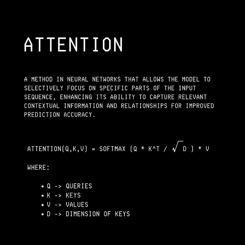
A type called the Scaled Dot-Product Attention was introduced in the Transformer architecture.
This is calculated using the following values:
Query (Q): a vector representing the current token that the model is processing.
Key (K): a vector representing each token in the sequence.
Value (V): a vector containing the information associated with each token.
This mechanism helps Transformers reach state-of-the-art performance on language tasks.
The question remained — Can they achieve such performance on Computer Vision tasks as well?
Vision Transformers Are Born
In 2021, a team of researchers from Google Brain applied the Transformer architecture directly to the sequences of image patches for image classification tasks.
They called their architecture — Vision Transformer or ViT.
This architecture follows the original Transformer implementation as closely as possible.
The input to a standard Transformer being trained for a language task is a 1D sequence of token embeddings.
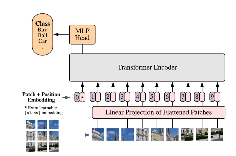
Similarly, to train a Transformer with images, these are first divided into fixed-size, non-overlapping patches.
Each patch is then flattened and linearly projected to create Patch embeddings.
Each patch is equivalent to a ‘token’ for the standard language tasked Transformer model.
These embeddings, along with Positional embeddings, are fed to the Encoder part of a Transformer, and its outputs are used to classify a given input image.
Let’s understand this process in more detail.
Exploring The Vision Transformer One Step At A Time
1. Creating Patch Embeddings
Say that each input image in the training dataset is of dimension H x W x C , where H , W and C represent the height, width, and channels.
Each image is flatted into N x (P² x C) patches, where (P, P) is each patch's resolution and N is the resulting number of patches.
Alternatively, one can also say that each patch is flattened into a vector of size P² x C.
Each patch is then mapped into a latent space of D dimensions using a trainable linear projection. This results in Patch embeddings.
2. Adding Positional Embeddings
Since the Transformer architecture is not sequential, learnable 1-D Positional embeddings are added to the Patch embeddings.

3. Adding The x(class) Token
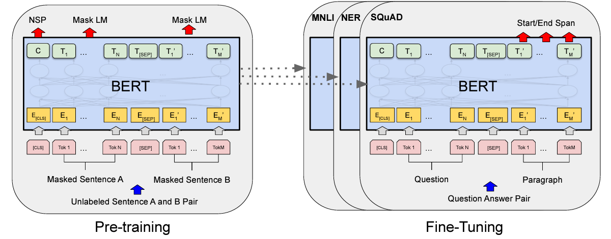
The next step borrows inspiration from the BERT architecture, where a special [CLS] token is added at the beginning of each input sequence.
This [CLS] token represents the entire input sequence, and its final hidden state representation C (shown in the image below) is used as an input for further classification tasks.
Similar to the above, an x(class) token is added to the sequence of Patch embeddings.
This token, after being processed by the L layers of the Transformer block is denoted as z(L) and captures the global representation of the entire image.
The previous equation is thus modified to the following:

This is the resulting input for the Transformer’s Encoder block.
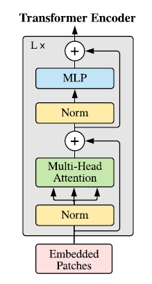
4. Feeding Embeddings To Transformer’s Encoder Block
Similar to the BERT architecture, only the Transformer’s Encoder block is used to process the embeddings.
This block consists of alternating layers of Multi-Head Attention and MLP blocks (consisting of two feed-forward layers with a GELU non-linearity).
Layer normalization (Norm) is applied before every block, and Residual connections (represented by the + sign in the image) are added after every block.
5. Adding A Classification Head
A Classification head processes the output z(L) from the Encoder.
This output is the compact representation of the entire image through the x(class) token.
During ViT’s pre-training, this classification head is an MLP with one hidden layer. However, during fine-tuning, it is simplified to a single linear layer.
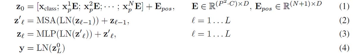
The following equations summarise how embeddings are transformed in the process.
Does Vision Transformer Perform Really Well?
Convolutional Neural Networks (CNNs) come with built-in biases that help them perform better with images.
These are:
Locality: The assumption that nearby image pixels are related.
2-D neighbourhood structure: The assumption that the 2D spatial arrangement of image pixels (height and width) matters towards an image’s meaning
Translation Equivariance: The assumption that if an object in an image shifts to another location, the features representing that object should shift similarly. In other words, the object’s identity won’t change just because it has moved to another location in the image.
Vision Transformers (ViTs) lack these built-in inductive biases.
ViTs use the Self-attention mechanism that treats each patch of an image independently without assuming any spatial patterns.
Thus, they have to learn how an image is structured from scratch.
Despite this, they absolutely smash the previous state-of-the-art models.
How do they achieve this?
ViTs learn the spatial structure of an image by learning the Positional embeddings of different patches during training.
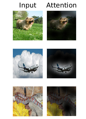
Their Multi-head attention mechanism allows some heads to focus on large sections of the image early on and others to focus on more minor and local details.
And, this attention mechanism overall captures and prioritizes the semantically important parts of an image.
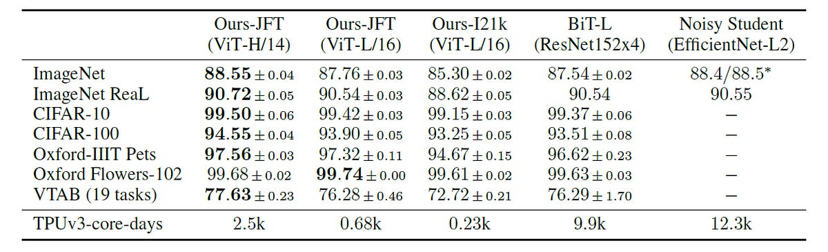
In the original research paper, ViT’s performance is compared against two leading CNN-based models:
Big Transfer (BiT): Based on ResNet that uses transfer learning through supervised pre-training
Noisy Student: Based on EfficientNet, trained using semi-supervised learning
The results show that ViTs not only exceed the performance of the baselines but also do so with reduced computational cost (evident with the lower TPUv3-core-days required for pre-training).
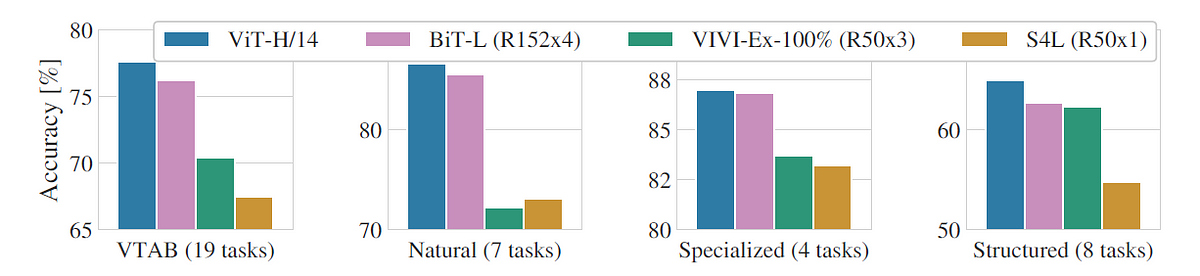
Vision Transformers (ViTs) also generalize well in their ability to classify images across natural, specialized, and structured domains as part of the Visual Task Adaptation (VTAB) benchmark.
Coding Up A Vision Transformer From Scratch
It’s time to implement what we have learned above.
Please note that I will not use the exact hyperparameters and datasets specified in the original research paper due to the significant computational cost involved with pre-training ViT.
The following ViT models of varying sizes are pre-trained in the original research paper.
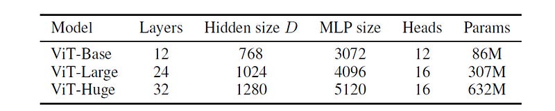
These models are pre-trained on large image datasets like ImageNet-21k and JFT-300M, and later fine-tuned to smaller, task-specific datasets such as CIFAR.
Instead of the above approach, we will pre-train our ViT model on the CIFAR-10 dataset.
The CIFAR-10 dataset consists of 60000 32 x 32 colour images in 10 classes, with 6000 images per class. There are 50000 training images and 10000 test images.
Step do this step by step.
1. Loading & Processing The Dataset
import torch
import torch.nn as nn
from torchvision import datasets, transforms
from torchvision.transforms import RandomErasing
from torch.utils.data import DataLoader

# Mean and standard deviation for CIFAR-10 dataset normalization
cifar10_mean = [0.4914, 0.4822, 0.4465]
cifar10_std  = [0.2023, 0.1994, 0.2010]

# Defining Transformations with data augmentation for Training images
transform_train = transforms.Compose([
    transforms.RandomCrop(32, padding=4),             # Randomly crop image to 32x32 with padding
    transforms.RandomHorizontalFlip(),                # Randomly flip image horizontally
    transforms.ToTensor(),                            # Convert PIL images to Tensor
    transforms.Normalize(cifar10_mean, cifar10_std),  # Normalize with CIFAR-10 mean and std
    RandomErasing(p=0.5, scale=(0.02, 0.33), ratio=(0.3, 3.3), value=0), #Randomly erase rectangle regions of the image
])

# Defining Transformations without data augmentation for Testing images
transform_test = transforms.Compose([
    transforms.ToTensor(),
    transforms.Normalize(cifar10_mean, cifar10_std),
])

# Loading CIFAR-10 dataset
train_dataset = datasets.CIFAR10(root='./data', train=True, download=True, transform=transform_train)
test_dataset = datasets.CIFAR10(root='./data', train=False, download=True, transform=transform_test)

# Creating efficient DataLoaders used for batching
train_loader = DataLoader(train_dataset, batch_size=128, shuffle=True, num_workers=2)
test_loader = DataLoader(test_dataset, batch_size=128, shuffle=False, num_workers=2)
Once the dataset is prepared, we define the Vision Transformer's components.
2. Defining The Patch Embedding Class
class PatchEmbedding(nn.Module):

    """
    Splits the image into patches and embeds them.

    Args:
        img_size (int): Size of the image.
        patch_size (int): Size of the patches.
        in_channels (int): Number of input channels (3 for RGB).
        emb_dim (int): Embedding dimension.

    Shape:
        - Input: (batch_size, in_channels, img_size, img_size)
        - Output: (batch_size, num_patches, emb_dim)
    """

    def __init__(self, img_size, patch_size, in_channels=3, emb_dim=256):
        super().__init__()

        self.patch_size = patch_size
        self.num_patches = (img_size // patch_size) ** 2

        # Linear projection layer
        self.linear_proj = nn.Linear(patch_size * patch_size * in_channels, emb_dim)


    def forward(self, x):

        """
        Forward pass for Patch embedding.

        Args:
            x: Input tensor of shape (batch_size, in_channels, img_size, img_size)

        Returns:
            Tensor of shape (batch_size, num_patches, emb_dim)
        """

        batch_size, channels, height, width = x.shape

        # Checks
        assert height == width, "Input images must be square."
        assert height % self.patch_size == 0, "Image dimensions must be divisible by the patch size."

        # Converting image into patches
        x = x.unfold(2, self.patch_size, self.patch_size)
        x = x.unfold(3, self.patch_size, self.patch_size)

        # x's shape: (batch_size, channels, num_patches_h, num_patches_w, patch_size, patch_size)

        num_patches_h = x.size(2)
        num_patches_w = x.size(3)

        # Flattening the patches
        x = x.permute(0, 2, 3, 1, 4, 5)  # x's shape: (batch_size, num_patches_h, num_patches_w, channels, patch_size, patch_size)
        x = x.reshape(batch_size, num_patches_h * num_patches_w, -1)  # x's shape: (batch_size, num_patches, patch_size * patch_size * channels)

        # Applying Linear projection to each patch
        x = self.linear_proj(x)  # x's shape: (batch_size, num_patches, emb_dim)

        return x
3. Defining The Multi-head Self Attention Class
class MultiHeadSelfAttention(nn.Module):
    """
    Multi-Head Self-Attention layer.

    Args:
        emb_dim (int): Embedding dimension.
        num_heads (int): Number of attention heads.

    Shape:
        - Input: (batch_size, num_patches + 1 (or seq_len), emb_dim)
        - Output: (batch_size, num_patches + 1 (or seq_len), emb_dim)
    """

    def __init__(self, emb_dim, num_heads):
        super().__init__()

        assert emb_dim % num_heads == 0,  "Embedding dimension must be divisible by num_heads."

        self.num_heads = num_heads
        self.head_dim = emb_dim // num_heads

        # Scaling factor for attention scores
        self.scale = self.head_dim ** -0.5

        # Linear layer to compute queries, keys, and values in one operation
        self.qkv = nn.Linear(emb_dim, emb_dim * 3)

        # Final linear layer to project concatenated outputs
        self.proj = nn.Linear(emb_dim, emb_dim)

    def forward(self, x):
        """
        Forward pass for multi-head self-attention.

        Args:
            x: Input tensor of shape (batch_size, seq_len, emb_dim)

        Returns:
            Output tensor of shape (batch_size, seq_len, emb_dim)
        """

        batch_size, seq_len, emb_dim = x.shape

        # Computing Queries, Keys, and Values
        qkv = self.qkv(x)

        # Splitting qkv into separate q, k, v tensors
        qkv = qkv.reshape(batch_size, seq_len, 3, self.num_heads, self.head_dim)
        qkv = qkv.permute(2, 0, 3, 1, 4)
        q, k, v = qkv[0], qkv[1], qkv[2]

        # Computing Attention scores
        attn_scores = torch.matmul(q, k.transpose(-2, -1))
        attn_scores = attn_scores * self.scale

        # Calculating Attention weights by applying Softmax
        attn_weights = attn_scores.softmax(dim=-1)

        # Scaling 'Value' by Attention weights
        attn_output = torch.matmul(attn_weights, v)

        # Concatenating attention outputs from all heads
        attn_output = attn_output.transpose(1, 2)
        attn_output = attn_output.reshape(batch_size, seq_len, emb_dim)

        # Applying final linear projection
        output = self.proj(attn_output)

        return output
4. Defining The Transformer Encoder Class
class TransformerEncoderLayer(nn.Module):
    """
    Transformer Encoder Layer with Multi-Head Self-Attention and MLP.

    Args:
        emb_dim (int): Embedding dimension.
        num_heads (int): Number of attention heads.
        mlp_dim (int): Dimension of the MLP hidden layer.
        dropout_rate (float): Dropout rate.

    Shape:
        - Input: (batch_size, num_patches + 1, emb_dim)
        - Output: (batch_size, num_patches + 1, emb_dim)
    """

    def __init__(self, emb_dim, num_heads, mlp_dim, dropout_rate=0.2):
        super().__init__()

        # Multi-Head Self-Attention
        self.msa = MultiHeadSelfAttention(emb_dim, num_heads)

        # MLP block
        self.mlp = nn.Sequential(
            nn.Linear(emb_dim, mlp_dim),
            nn.GELU(),
            nn.Dropout(dropout_rate),
            nn.Linear(mlp_dim, emb_dim),
            nn.Dropout(dropout_rate),
        )

        # Layer Normalization
        self.norm1 = nn.LayerNorm(emb_dim)
        self.norm2 = nn.LayerNorm(emb_dim)

    def forward(self, x):
        """
        Forward pass for the Transformer Encoder Layer.

        Args:
            x: Input tensor of shape (batch_size, num_patches + 1, emb_dim)

        Returns:
            Tensor of shape (batch_size, num_patches + 1, emb_dim)
        """

        # Applying Layer Normalization and Multi-Head Self-Attention with Residual connection
        x = x + self.msa(self.norm1(x))

        # Applying Layer Normalization and MLP block with Residual connection
        x = x + self.mlp(self.norm2(x))

        return x
5. Defining The Vision Transformer Class
class VisionTransformer(nn.Module):
      """
      Vision Transformer (ViT) Model.

      Args:
          img_size (int): Size of the input image.
          patch_size (int): Size of each patch.
          in_channels (int): Number of input channels.
          emb_dim (int): Embedding dimension.
          num_layers (int): Number of Transformer encoder layers.
          num_heads (int): Number of attention heads.
          mlp_dim (int): Dimension of the MLP hidden layer.
          num_classes (int): Number of output classes.
          dropout_rate (float): Dropout rate.

      Shape:
          - Input: (batch_size, in_channels, img_size, img_size)
          - Output: (batch_size, num_classes)
      """
      def __init__(
        self, img_size, patch_size, in_channels, emb_dim, num_layers,
        num_heads, mlp_dim, num_classes, dropout_rate):
        super().__init__()

        # Patch Embedding
        self.patch_embed = PatchEmbedding(img_size, patch_size, in_channels, emb_dim)

        # Learnable class token (x_class)
        self.class_token = nn.Parameter(torch.zeros(1, 1, emb_dim))

        # Learnable Positional Embedding
        num_patches = self.patch_embed.num_patches
        self.pos_embed = nn.Parameter(torch.zeros(1, num_patches + 1, emb_dim))

        # Dropout layer
        self.dropout = nn.Dropout(dropout_rate)

        # Transformer Encoder Layers
        self.encoder_layers = nn.ModuleList([
            TransformerEncoderLayer(emb_dim, num_heads, mlp_dim, dropout_rate)
            for _ in range(num_layers)
        ])

        # Final Layer Normalization
        self.norm = nn.LayerNorm(emb_dim)

        # Classification Head (MLP with one hidden layer)
        self.hidden_dim = emb_dim

        self.classifier = nn.Sequential(
            nn.Linear(emb_dim, self.hidden_dim),
            nn.GELU(),
            nn.Dropout(dropout_rate),
            nn.Linear(self.hidden_dim, num_classes)
        )

    def forward(self, x):
        """
        Forward pass for the Vision Transformer.

        Args:
            x: Input tensor of shape (batch_size, in_channels, img_size, img_size)

        Returns:
            Tensor of shape (batch_size, num_classes)
        """

        batch_size = x.shape[0]

        # Applying Patch Embedding
        x = self.patch_embed(x)

        # Adding class token
        class_token = self.class_token.expand(batch_size, -1, -1)
        x = torch.cat((class_token, x), dim=1)

        # Adding Positional embeddings
        x = x + self.pos_embed

        # Applying Dropout
        x = self.dropout(x)

        # Pass through Transformer Encoder
        for layer in self.encoder_layers:
            x = layer(x)

        # Step 5: Apply final LayerNorm
        x = self.norm(x)

        # Extracting the class token
        cls_token_final = x[:, 0]

        # Pass through the Classification head
        logits = self.classifier(cls_token_final)

        return logits
Once we have defined the Vision Transformer, let’s write the code to train and evaluate it.
6. Defining The Training & Evaluation Functions
# Training function

def train(model, dataloader, optimizer, criterion, device):
    """
    Training loop for one epoch.

    Args:
        model: The neural network model.
        dataloader: DataLoader for the training data.
        optimizer: Optimizer for updating model parameters.
        criterion: Loss function.
        device: Device to perform computations on (CPU or GPU).

    Returns:
        Tuple of average loss and accuracy over the epoch.
    """
    model.train()

    total_loss = 0
    total_correct = 0
    total_samples = 0

    loop = tqdm(dataloader, leave=True)

    for images, labels in loop:
        images, labels = images.to(device), labels.to(device)
        batch_size = images.size(0)

        optimizer.zero_grad()

        # Forward pass
        outputs = model(images)

        # Computing loss
        loss = criterion(outputs, labels)

        # Backward pass and optimization
        loss.backward()
        optimizer.step()

        # Updating metrics
        total_loss += loss.item() * batch_size
        _, predicted = torch.max(outputs.data, 1)
        total_correct += (predicted == labels).sum().item()
        total_samples += batch_size

        # Updating the progress bar
        loop.set_description(f"Training - Loss: {total_loss / total_samples:.4f}, Accuracy: {total_correct / total_samples:.4f}")

    avg_loss = total_loss / total_samples
    avg_acc = total_correct / total_samples

    return avg_loss, avg_acc
# Evaluation function
def evaluate(model, dataloader, criterion, device):
"""
Evaluation loop for one epoch.
Args:
model: The neural network model.
dataloader: DataLoader for the validation/test data.
criterion: Loss function.
device: Device to perform computations on (CPU or GPU).
Returns:
Tuple of average loss and accuracy over the epoch.
"""
model.eval()
total_loss = 0
total_correct = 0
total_samples = 0
loop = tqdm(dataloader, leave=True)
with torch.no_grad():
for images, labels in loop:
images, labels = images.to(device), labels.to(device)
batch_size = images.size(0)
# Forward pass
outputs = model(images)
# Computing loss
loss = criterion(outputs, labels)
# Updating metrics
total_loss += loss.item() * batch_size
_, predicted = torch.max(outputs.data, 1)
total_correct += (predicted == labels).sum().item()
total_samples += batch_size
# Updating the progress bar
loop.set_description(f"Evaluating - Loss: {total_loss / total_samples:.4f}, Accuracy: {total_correct / total_samples:.4f}")
avg_loss = total_loss / total_samples
avg_acc = total_correct / total_samples
return avg_loss, avg_accLet’s finally train the model on the dataset.
7. Training The ViT
# Instantiating the Vision Transformer model
model = VisionTransformer(
    img_size=32,       # CIFAR-10 image size
    patch_size=4,      # Each patch will be 4x4 pixels
    in_channels=3,     # RGB images have 3 channels
    emb_dim=256,       # Embedding dimension
    num_layers=4,      # Number of Transformer encoder layers
    num_heads=4,       # Number of attention heads
    mlp_dim=128,       # Dimension of the MLP in encoder layers
    num_classes=10,    # CIFAR-10 has 10 classes
    dropout_rate=0.2   # Dropout rate
)

# Setting device to GPU if available
device = torch.device("cuda" if torch.cuda.is_available() else "cpu")
model.to(device)

print("Training on: ", device)

# Defining optimizer, loss function, and learning rate scheduler
optimizer = optim.AdamW(model.parameters(), lr=3e-4, weight_decay=0.01)
scheduler = optim.lr_scheduler.CosineAnnealingWarmRestarts(optimizer, T_0=10, T_mult=2)
criterion = nn.CrossEntropyLoss(label_smoothing=0.1)

# Lists to store metrics for plotting
train_losses = []
train_accuracies = []
val_losses = []
val_accuracies = []

# Number of training epochs
num_epochs = 100

# Early Stopping
best_val_loss = float("inf")
patience = 5
trigger_times = 0

for epoch in range(num_epochs):
    print(f"Epoch {epoch + 1}/{num_epochs}")

    # Training loop
    train_loss, train_acc = train(model, train_loader, optimizer, criterion, device)

    # Evaluation loop
    val_loss, val_acc = evaluate(model, test_loader, criterion, device)

    # Updating the learning rate scheduler
    scheduler.step()

    # Storing the metrics
    train_losses.append(train_loss)
    train_accuracies.append(train_acc)
    val_losses.append(val_loss)
    val_accuracies.append(val_acc)

    # Printing epoch results
    print(f"Train Loss: {train_loss:.4f}, Train Accuracy: {train_acc * 100:.2f}%")
    print(f"Validation Loss: {val_loss:.4f}, Validation Accuracy: {val_acc * 100:.2f}%\n")

    # Check for early stopping
    if val_loss < best_val_loss:
        best_val_loss = val_loss
        trigger_times = 0
        # Optionally save the model checkpoint
        torch.save(model.state_dict(), 'best_model.pt')
    else:
        trigger_times += 1
        print(f'EarlyStopping counter: {trigger_times} out of {patience}')
        if trigger_times >= patience:
            print('Early stopping!')
            break
The hyperparameters used above were based on trial and error, and I realised that using the following were leading to poor performance and overfitting:
larger
emb_dim,mlp_dim,num_layers,num_headssmall
dropout_rateusing
Adaminstead ofAdamWupscaling CIFAR-10 images to 224 x 224 for training (as in the original ViT architecture)
using
nn.CrossEntropyLossloss without label smoothingusing
CosineAnnealingLRinstead ofCosineAnnealingWarmRestartsfor learning rate scheduling
I also used Early Stopping in the above example.
8. Plotting The Training and Validation Curves
# Finding the actual number of epochs completed
num_epochs_completed = len(train_losses)
epochs = range(1, num_epochs_completed + 1)

# Plotting Training and Validation Loss
plt.figure(figsize=(10, 4))
plt.plot(epochs, train_losses, label='Training Loss')
plt.plot(epochs, val_losses, label='Validation Loss')
plt.title('Training and Validation Loss')
plt.xlabel('Epochs')
plt.ylabel('Loss')
plt.legend()
plt.grid(True)
plt.show()

# Plotting Training and Validation Accuracy
plt.figure(figsize=(10, 4))
plt.plot(epochs, train_accuracies, label='Training Accuracy')
plt.plot(epochs, val_accuracies, label='Validation Accuracy')
plt.title('Training and Validation Accuracy')
plt.xlabel('Epochs')
plt.ylabel('Accuracy')
plt.legend()
plt.grid(True)
plt.show()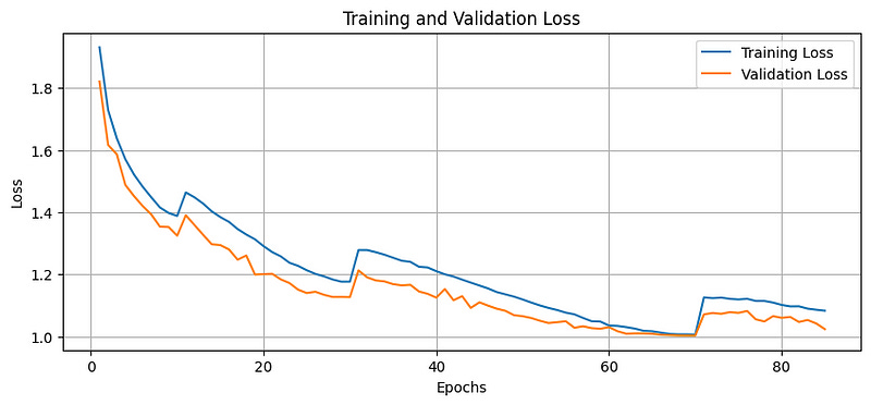
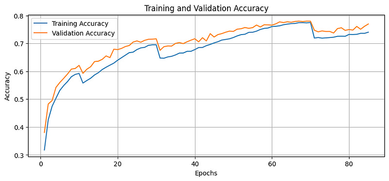
As noted with these plots, the training and validation loss decreases, and the accuracy improves over the epochs until the 85th epoch (beyond which Early Stopping is triggered).
The validation loss also remains below the training loss, indicating that the model does not overfit during these epochs.
9. Visualising The Results
Let’s finally see how well the model predicts the CIFAR-10 images.
# Function to plot image predictions

def plot_predictions(model, dataloader, device, classes, num_images=9):
    """
    Plots a grid of images from the dataloader with actual and predicted labels.

    Args:
        model: Trained neural network model.
        dataloader: DataLoader for the dataset to plot images from.
        device: Device to perform computations on.
        classes: List of class names.
        num_images: Number of images to display.

    Displays:
        A grid of images with actual and predicted labels.
    """

    model.eval()
    images_shown = 0
    cols = 3
    rows = num_images // cols + int(num_images % cols > 0)
    plt.figure(figsize=(5, 2 * rows))

    with torch.no_grad():
        for images, labels in dataloader:
            images, labels = images.to(device), labels.to(device)
            outputs = model(images)
            _, preds = torch.max(outputs, 1)

            for idx in range(images.size(0)):
                if images_shown >= num_images:
                    break
                image = images[idx].cpu().numpy()
                image = np.transpose(image, (1, 2, 0))

                # Unnormalizing the image
                mean = np.array(cifar10_mean)
                std = np.array(cifar10_std)
                image = std * image + mean
                image = np.clip(image, 0, 1)

                actual_label = classes[labels[idx].item()]
                predicted_label = classes[preds[idx].item()]

                ax = plt.subplot(rows, cols, images_shown + 1)
                plt.imshow(image)
                plt.title(f"Actual: {actual_label}\nPredicted: {predicted_label}")
                plt.axis('off')

                images_shown += 1

            if images_shown >= num_images:
                break
    plt.tight_layout()
    plt.show()

# CIFAR-10 class labels
classes = ['airplane', 'automobile', 'bird', 'cat', 'deer',
           'dog', 'frog', 'horse', 'ship', 'truck']

# Plotting the prediction
plot_predictions(model, test_loader, device, classes, num_images=9)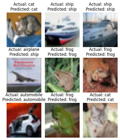
We can see that the ViT predictions match the actual image labels for most images.
That’s everything for this tutorial on Vision Transformers. I’d love to know your results if you train one from scratch.
Happy learning!
Further Reading