
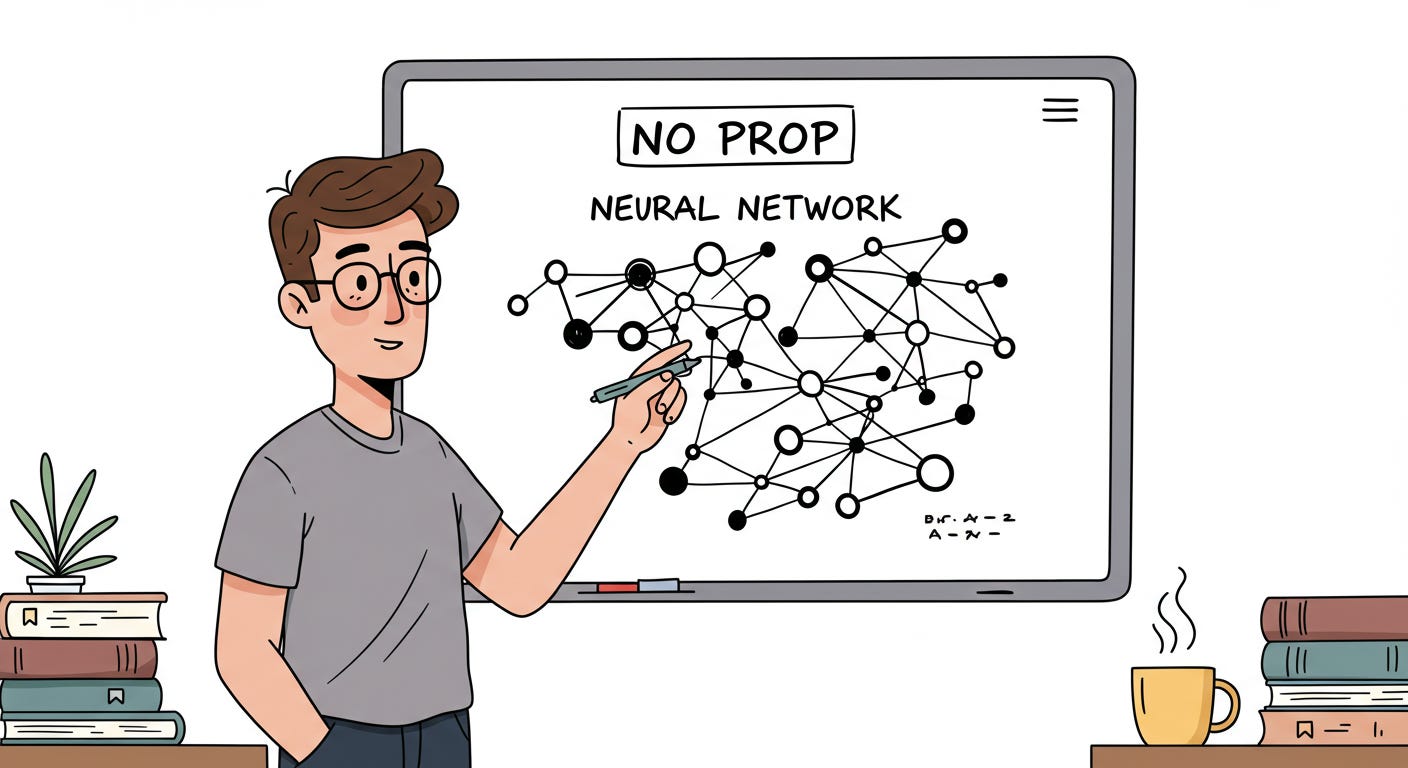
You Don't Need Backpropagation To Train Neural Networks Anymore
A deep dive into the 'NoProp' algorithm that eliminates the need for Forward pass and Backpropagation to train neural networks, and learning to code it from scratch.

Backpropagation, first introduced in 1986, is one of the critical algorithms that underlie the training of all popular ML models that we use today.
It is simple, easy to implement and effective in training large neural networks.
Although widely accepted as the best method for this, it comes with some disadvantages, including high memory usage during training and difficulty in parallelising training due to the sequential nature of the algorithm.
Is there an algorithm that can still train neural networks effectively, and comes without these disadvantages?
A team of researchers from the University of Oxford has just introduced one that eliminates the need for backpropagation.
Their algorithm, called NoProp, does not even require a Forward pass and works on the principles followed by Diffusion models to train each layer of a neural network independently without passing gradients.
Here is a story where we take a deep dive into how this algorithm works, learn about its comparative performance, and learn to code it from scratch to train our own neural network.
Let’s begin!
But First, What Is Backpropagation?
MLPs or Multi-Layer Perceptrons are fully connected feed-forward deep neural networks that are at the core of all AI technology that we see today.
They consist of units called Neurons.

Neurons are stacked up in multiple layers, and each neuron in one layer is connected to every neuron in the next layer in MLPs.

During training, input data is passed through these neural networks, with each layer applying weights, biases, and activation functions to it, modifying the data sequentially and producing an output/ prediction at the final layer.
This step is called the Forward pass or Forward propagation.

Following this, the output prediction from the forward pass is compared to the actual label associated with the input data, and an error or loss function is calculated.
This is where the Backpropagation algorithm comes in, which computes the gradient of the loss with respect to the network's parameters (weights and biases), iterating backwards from the last layer.
This is done via the chain rule in calculus and tells us how much each parameter contributes to the error (Credit assignment).
This step is called the Backward pass.
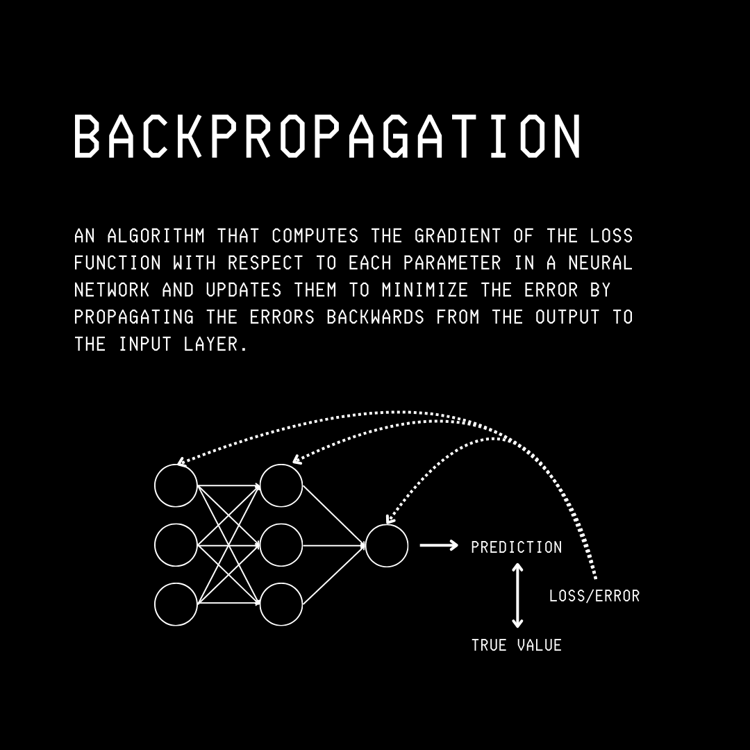
After backpropagation, an optimiser updates/ adjusts these parameters, layer by layer, to reduce the loss, leading to a better model.
But What’s Wrong With Backpropagation?
Although highly effective, Backpropagation is memory-intensive.
Remember all the outputs produced by each hidden layer during the forward pass? These are also referred to as Intermediate activations, and these must be stored because they are all needed later in the backward pass.
For neural networks with hundreds of layers and millions of neurons, storing intermediate activations during training can consume multiple GBs of GPU VRAM.
(Techniques like Gradient checkpointing have been developed to address this issue, but this still remains a significant expense.)
Also, because Backpropagation is a sequential algorithm, the computation of gradients for each layer depends on the gradients from the subsequent layer.
This means that we cannot run all gradient calculations simultaneously by parallelising them across layers, and each layer must wait for the gradients from the layer after it before proceeding with its own gradient calculation.
Neural networks trained by Backpropagation also learn things hierarchically, which means that learning is organised across multiple levels of abstraction, where lower layers learn simple patterns and higher layers build on them to learn more complex ones.
When gradients are propagated backwards through these networks, updates from one data point or task can interfere with updates from others, causing the networks to sometimes completely forget previously learned data (a phenomenon known as Catastrophic Forgetting).
The following methods are a few of the many that have been previously developed as alternatives to backpropagation but have not gained much success.
This is due to them being low in accuracy, computational efficiency, reliability, or scalability.
Is effective backpropagation-free learning still possible then?
Here Comes ‘NoProp’
The NoProp algorithm borrows insights from Diffusion models (primarily used for image generation tasks) and applies them to an Image classification (supervised learning) task.
If you’re short on time and want to skip the mathematical details, this is how the algorithm works in short.
During training, each layer/ block in a neural network is given a noisy label and a training input, and it predicts the target label based on these.
Each layer is trained independently of other layers using a denoising loss. This eliminates the need for a Forward pass during training time.
Unlike training, all the layers work together during inference.
Starting from Gaussian noise, each layer takes a noisy label produced by the previous layer and denoises it.
This is progressively done layer by layer, with the network returning the true class (the fully denoised representation) from the final layer.
Let’s now explore the inner workings of this algorithm in detail.
(You will be able to understand this much better if you are already familiar with Diffusion models.)
Given a sample input x and its label y from a dataset, our goal is to build a model that can predict the label y given input x.
Mathematically, instead of finding a function f(x) = y, we want to train a neural network to model a stochastic process that transforms random noise into a form that allows us to estimate y.
Two distributions are important to understand in this process:
1. Stochastic Forward/ Denoising Process
This process is represented by p as shown below:

It models how we can start with noise and, through a series of steps, denoise it toward the final representation z(T), which is then used to predict the label y.
Mathematically, it is the joint probability of all intermediate noisy representations z(0), …, z(T) and the label y, given x.
In the equation:
p(z(0))describes the standard Gaussian noisep(z(t) ∣ z(t−1), x)describes how each layer denoises the input noisep(y ∣ z(T))describes howyis classified based on the final representationz(T)
p(z(t) ∣ z(t−1), x) is parameterized using a neural network as follows:

where:
neural network
ûwith parametersθ, weighted bya(t), predicts the denoised representation based on the noisy inputsz(t-1)andxb(t) ⋅ z(t−1)represents a weighted skip connection√c(t) ⋅ ϵ(t)represents random Gaussian noisea(t),b(t),c(t)are scalers that are used to weigh the three different parts of the equation
2. Backward Noising Process/ Variational Posterior
This process is represented by q as shown below:

It models how we can start with a label y (in the form of its embedding u(y)) and add noise step by step until we get the noise z(0).
Mathematically, it is the probability of the final noisy representation z(T) given the label y and input x.
In the equation:
q(z(T) ∣ y)describes the representationz(T)given labelyxq(z(t−1) ∣ z(t))describes the reverse diffusion process of reaching earlier noisy representations by adding more noise
q(z(T) ∣ y) is given using the following equation:

This means that it is a Gaussian distribution over the latent variable z(T) where √αˉ(T)⋅ u(y) is the mean and 1 — αˉ(T) is the variance.
u(y) is the label embedding and αˉ(T) tells how much of u(y) remains after applying the noising process.
q(z(t−1) ∣ z(t)) is given by the following equation:

This means that it is a Gaussian distribution over the latent variable z(t-1) where √α(t-1)⋅ z(t) is the mean and 1 — α(t-1) is the variance.
α(t−1) is a noise scheduling parameter that controls how much of the original signal is preserved at timestep t-1.
Note that the terms α and αˉ come from a fixed cosine noise schedule.
Defining The Loss
The training objective of the NoProp algorithm is to maximise the log-likelihood of the correct label log p(y∣x).
But directly optimising this log-likelihood is mathematically difficult, so as a workaround, we instead maximise a variational lower bound on it called the Evidence Lower Bound (ELBO).


The NoProp loss is derived from this expression as:

(The mathematical details of this derivation are described in Section A.4 of the original research paper.)
This looks very complex, but is easy to understand.
On the right-hand side of the equation:
The first term is the Cross-entropy loss, which measures how accurately the final representation
z(T)can be used to predict the correct labely.The second term is the Kullback-Leibler (KL) divergence between the distribution of the starting representation
z(0)and the standard Gaussian noise distribution. This regularization encourages both of these distributions to be similar, which is necessary for the diffusion process to work properly.The third term is the layer-wise Denoising loss, which measures how well each layer denoises by comparing how close its output is to the true label embedding (given by the L2 loss term).
In the equation, η is a hyperparameter and the term SNR is the Signal-to-Noise Ratio, given by the following equation:

As t increases (as we move towards the later layers), the signal increases (noise decreases) and hence SNR increases. This makes the overall denoising loss larger.
This means that the model is penalized more for errors from the later layers (t closer to T) than the earlier ones.
Training Process
During training, the network learns to denoise noisy label embeddings at each layer, without doing a full forward or backward pass through the network.
For a given input-label pair (x, y) an embedding matrix W(embed) maps the labels y to embeddings u(y) with each row of this matrix corresponding to the embedding u(y) of the label y.
Noise is first added to u(y) to create z(t).
Then, each neural network layer û(θ)(z(t−1) , x) is trained independently to denoise the previous noisy representation z(t-1) by predicting the clean embedding u(y) using input x.
The training loss is calculated, and the network parameters are updated while minimising this loss, using an optimiser.
The training algorithm is summarised using the pseudocode shown below.

Inference Process
During inference, the network with T total layers/ blocks is given Gaussian noise z(0).
Each layer, starting from Gaussian noise z(0), sequentially takes the output z(t-1) from the previous layer, and input x, to produce the next denoised representation z(t).
This results in a sequence of intermediate forms of the noise at each layer, represented by z(0), z(1), …, z(t), z(T-1), z(T).
At the final step t = T, the output z(T) is passed through a classifier to predict the final label ŷ.

ŷ.Layer/ Block Architecture
Each layer/ block û(θ)(z(t−1) , x), as described above, is a complex neural network in itself that takes:
the input
xand processes it through a convolutional embedding module, followed by a fully connected layernoised representation from the previous layer
z(t-1), and processes it using a fully connected network with skip connections
These inputs are then passed through additional fully connected layers to produce logits.
The logits go through a softmax function, producing a probability distribution over class embeddings.
The final output is obtained by computing a weighted sum of the class embeddings using this probability distribution.

How Well Does NoProp Perform?
What we described above was the Discrete-Time (DT) variant of NoProp called NoProp-DT.
This is called so because it is implemented to model the diffusion process in discrete time steps, rather than continuously.
There are two other variants of it, namely:
NoProp-CT (Continuous-Time): This variant uses a continuous noise schedule and models the diffusion process over a continuous time span instead of discrete steps.
NoProp-FM (Flow Matching): This variant learns the vector field that transports noise towards the predicted label embedding via an ordinary differential equation (ODE), rather than the denoising approach.
All of these variants are compared with backpropagation and previous backpropagation-free methods for image classification tasks on three benchmark datasets:
MNIST: A dataset of 70,000 grayscale images of handwritten digits (each 28 x 28 pixels), across 10 classes (digits 0–9)
CIFAR-10: A dataset of 60,000 color images (each 32 x 32 pixels) across 10 different object classes
CIFAR-100: A dataset of 60,000 color images (each 32 x 32 pixels) across 100 different object classes
Experiments show that NoProp achieves performance comparable to or better than backpropagation and other backpropagation-free methods on all three datasets.

Alongside this, NoProp consumes less GPU memory during training as compared to other methods.

Coding No-Prop From Scratch
Now that we know the theory behind NoProp, let’s learn to code it ourselves and test the results.
All the code is written using PyTorch in a Jupyter notebook, making it easier to follow and run.
Installing Dependencies
You will not need to install these if you’re using a Google Colab notebook to run this code.
!uv pip install torch torchvision matplotlibUsing GPU/ Apple MPS If Available
# Set device

if torch.backends.mps.is_available():
    device = "mps"
elif torch.cuda.is_available():
    device = "cuda"
else:
    device = "cpu"

print("Using device:", device)
Defining The Denoising Block
This is the denoising neural network block (û(θ)) that takes:
an image
xa noisy intermediate representation
z(t-1), andthe class embedding matrix
W_embedthat contains label embeddingsu(y)as its rows
It then learns to denoise the noisy latent vector z(t-1) and bringing it closer to the true label embedding u(y) using information from the image x.
It returns the next representation z(t) given these inputs.
Unlike conventional neural networks, each of these blocks independently learn to remove noise towards the label embedding.
# Denoising block

class DenoiseBlock(nn.Module):
    def __init__(self, embedding_dim, num_classes):
        super().__init__()
        # Image path
        self.conv_path = nn.Sequential(
            nn.Conv2d(1, 32, 3, padding=1),
            nn.ReLU(),
            nn.MaxPool2d(2),
            nn.Dropout(0.2),
            nn.Conv2d(32, 64, 3, padding=1),
            nn.ReLU(),
            nn.Dropout(0.2),
            nn.Conv2d(64, 128, 3, padding=1),
            nn.ReLU(),
            nn.MaxPool2d(2),
            nn.Dropout(0.2),
            nn.AdaptiveAvgPool2d((1, 1)),
            nn.Flatten(),
            nn.Linear(128, 256),
            nn.BatchNorm1d(256)
        )

        # Noisy embedding path
        self.fc_z1 = nn.Linear(embedding_dim, 256)
        self.bn_z1 = nn.BatchNorm1d(256)

        self.fc_z2 = nn.Linear(256, 256)
        self.bn_z2 = nn.BatchNorm1d(256)

        self.fc_z3 = nn.Linear(256, 256)
        self.bn_z3 = nn.BatchNorm1d(256)

        # Combined downstream path
        self.fc_f1 = nn.Linear(256 + 256, 256)
        self.bn_f1 = nn.BatchNorm1d(256)
        self.fc_f2 = nn.Linear(256, 128)
        self.bn_f2 = nn.BatchNorm1d(128)
        self.fc_out = nn.Linear(128, num_classes)

    def forward(self, x, z_prev, W_embed):
        # Image features
        x_feat = self.conv_path(x)

        # Features from noisy embedding
        h1 = F.relu(self.bn_z1(self.fc_z1(z_prev)))
        h2 = F.relu(self.bn_z2(self.fc_z2(h1)))
        h3 = self.bn_z3(self.fc_z3(h2))

        z_feat = h3 + h1 # Residual connection

        # Combine and predict logits
        h_f = torch.cat([x_feat, z_feat], dim=1)
        h_f = F.relu(self.bn_f1(self.fc_f1(h_f)))
        h_f = F.relu(self.bn_f2(self.fc_f2(h_f)))
        logits = self.fc_out(h_f)

        # Softmax on logits
        p = F.softmax(logits, dim=1)
        z_next = p @ W_embed

        return z_next, logits
Defining The NoProp-DT Model
This model combines the label denoising through a T-step diffusion process, using independently trained DenoiseBlocks.
# NoProp-DT model

class NoPropDT(nn.Module):
    def __init__(self, num_classes, embedding_dim, T, eta):
        super().__init__()
        self.num_classes = num_classes
        self.embedding_dim = embedding_dim
        self.T = T
        self.eta = eta

        # Stacking up the Denoise blocks
        self.blocks = nn.ModuleList([
            DenoiseBlock(embedding_dim, num_classes) for _ in range(T)
        ])

        # Class-embedding matrix (W_embed)
        self.W_embed = nn.Parameter(torch.randn(num_classes, embedding_dim) * 0.1)

        # Classification head
        self.classifier = nn.Linear(embedding_dim, num_classes)

        # Cosine noise schedule
        t = torch.arange(1, T+1, dtype=torch.float32)
        alpha_t = torch.cos(t / T * (math.pi/2))**2
        alpha_bar = torch.cumprod(alpha_t, dim=0)
        snr = alpha_bar / (1 - alpha_bar)
        snr_prev = torch.cat([torch.tensor([0.], dtype=snr.dtype), snr[:-1]], dim=0)
        snr_diff = snr - snr_prev

        self.register_buffer('alpha_bar', alpha_bar)
        self.register_buffer('snr_diff', snr_diff)

    def forward_denoise(self, x, z_prev, t):
        return self.blocks[t](x, z_prev, self.W_embed)[0]

    def classify(self, z):
        return self.classifier(z)

    def inference(self, x):
        B = x.size(0)
        z = torch.randn(B, self.embedding_dim, device=x.device)

        for t in range(self.T):
            z = self.forward_denoise(x, z, t)

        return self.classify(z)
Defining The Training Function
This function trains the NoProp-DT model (creating by combining T Denoising blocks without using backpropagation.
# Function for training NoProp-DT

def train_nopropdt(model, train_loader, test_loader, epochs, lr, weight_decay):
    # Using AdamW optimizer
    optimizer = torch.optim.AdamW(model.parameters(), lr=lr, weight_decay=weight_decay)

    # Dict to store metrics
    history = {'train_acc': [], 'val_acc': []}

    for epoch in range(1, epochs + 1):
        model.train()

        for t in range(model.T):
            for x, y in train_loader:
                x, y = x.to(device), y.to(device)
                uy = model.W_embed[y]
                alpha_bar_t = model.alpha_bar[t]
                noise = torch.randn_like(uy)
                z_t = torch.sqrt(alpha_bar_t) * uy + torch.sqrt(1 - alpha_bar_t) * noise

                z_pred, _ = model.blocks[t](x, z_t, model.W_embed)
                loss_l2 = F.mse_loss(z_pred, uy)
                loss = 0.5 * model.eta * model.snr_diff[t] * loss_l2

                if t == model.T - 1:
                    logits = model.classifier(z_pred)
                    loss_ce = F.cross_entropy(logits, y)
                    loss_kl = 0.5 * uy.pow(2).sum(dim=1).mean()
                    loss = loss + loss_ce + loss_kl

                optimizer.zero_grad()
                loss.backward()
                torch.nn.utils.clip_grad_norm_(model.parameters(), 1.0)
                optimizer.step()

        # Training accuracy
        model.eval()
        correct, total = 0, 0
        with torch.no_grad():
            for x, y in train_loader:
                x, y = x.to(device), y.to(device)
                preds = model.inference(x).argmax(dim=1)
                correct += (preds == y).sum().item()
                total += y.size(0)

        train_acc = correct / total

        # Validation accuracy
        val_correct, val_total = 0, 0
        with torch.no_grad():
            for x, y in test_loader:
                x, y = x.to(device), y.to(device)
                preds = model.inference(x).argmax(dim=1)
                val_correct += (preds == y).sum().item()
                val_total += y.size(0)

        val_acc = val_correct / val_total

        # Storing accuracy history
        history['train_acc'].append(train_acc)
        history['val_acc'].append(val_acc)

        print(f"Epoch {epoch}/{epochs}  "
              f"TrainAcc={100 * train_acc:.2f}%  ValAcc={100 * val_acc:.2f}%")

    # Plotting Training and Validation accuracy
    plt.figure()
    plt.plot(range(1, epochs + 1), history['train_acc'], label='Train Accuracy')
    plt.plot(range(1, epochs + 1), history['val_acc'], label='Validation Accuracy')
    plt.title("Accuracy Curve")
    plt.xlabel("Epoch")
    plt.ylabel("Accuracy")
    plt.legend()
    plt.grid(True)
    plt.show()

    print(f"\n Final Test Accuracy: {100 * val_acc:.2f}%")
Defining Hyperparameters
The hyperparameters used by the authors in their experiments are shown below.
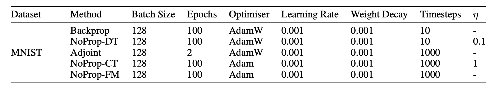
There’s just a minor change: we're training the model for only 10 epochs instead of 100, as this amount of training is sufficient to achieve satisfactory results for our tutorial.
# Hyperparameters

T = 10
eta = 0.1
embedding_dim = 512
batch_size = 128
lr = 1e-3
epochs = 10
weight_decay = 1e-3
Loading MNIST Dataset
We will not apply data augmentation techniques on the MNIST dataset. This is similar to the experiments from the original research paper.
# Loading MNIST

transform = transforms.ToTensor()

train_set = torchvision.datasets.MNIST(root='./data', train=True, download=True, transform=transform)
test_set  = torchvision.datasets.MNIST(root='./data', train=False, download=True, transform=transform)

train_loader = DataLoader(train_set, batch_size=batch_size, shuffle=True)
test_loader  = DataLoader(test_set,  batch_size=batch_size)
Initializing The Model
Let’s set up the model with the hyperparameters that we defined.
# Initializing model

model = NoPropDT(num_classes=10, embedding_dim=embedding_dim, T=T, eta=eta).to(device)
Training The Model
It’s time to start training!
# Begin training

train_nopropdt(model, train_loader, test_loader, epochs=epochs, lr=lr, weight_decay=weight_decay)
At the end of training, we get a 98.88% Validation accuracy!

Visualising Predictions
Let’s plot these predictions and visualise the results.
# Function to plot predictions

def show_predictions(model, test_loader, class_names=None, num_images = 16):
    model.eval()
    images_shown = 0
    plt.figure(figsize=(5, 5))

    with torch.no_grad():
        for x, y in test_loader:
            x, y = x.to(device), y.to(device)
            logits = model.inference(x)
            preds = logits.argmax(dim=1)

            for i in range(x.size(0)):
                if images_shown >= num_images:
                    break

                plt.subplot(int(num_images**0.5), int(num_images**0.5), images_shown + 1)
                img = x[i].cpu().squeeze(0)
                plt.imshow(img, cmap='gray')
                actual = class_names[y[i]] if class_names else y[i].item()
                pred = class_names[preds[i]] if class_names else preds[i].item()
                plt.title(f"Pred: {pred}\nTrue: {actual}", fontsize=8)
                plt.axis('off')

                images_shown += 1

            if images_shown >= num_images:
                break

    plt.tight_layout()
    plt.show()
# Class names for MNIST dataset
class_names = [str(i) for i in range(10)]
# Visualising predictions
show_predictions(model, test_loader)
That’s all about this tutorial on the NoProp algorithm.
What are your thoughts on it? Share your results with me in the comments below if you train a neural network using it!
Further Reading
Notebook containing the code for training a neural network with NoProp-DT on the MNIST dataset
Research paper titled ‘Denoising Diffusion Probabilistic Models’ published in ArXiv
Research paper titled ‘Learning representations by back-propagating errors’ published in Nature
Source Of Images
All images, including the screenshots used in the article, are either created by the author or obtained from the original research paper unless stated otherwise.

Oh hey I appreciate you looking at and liki.g my comment. Upon publishing I realized my LaTex embeddings were missing. I have added the ones I think I had in there. If you want to revisit the article for clarity it's under sect IV mathmatical and structural interpretation to give you a window into the application
I'm working on a patent for a novel a.i model. I just wrote an article about the concepts in employing. The article is not technical as I am working on the patent that explains the how, but if interested please read the article as it still has value in some novel concepts .
https://open.substack.com/pub/theeoutlier/p/semantic-resonance-and-fractal-scale?r=3nhnfp&utm_campaign=post&utm_medium=web