
Meta’s Large Concept Models (LCMs) Are Here To Challenge And Redefine LLMs
A deep dive into ‘Large Concept Model’, a novel language processing architecture and evaluating its performance against state-of-the-art LLMs

LLMs, or Large Language Models, are dominating all language-based tasks today.
Alongside language tasks, their extension to images, video, and speech has led to state-of-the-art performance as well.
Most LLMs are based on the Decoder-only Transformer architecture.
This architecture is trained to predict the next token based on the context of preceding tokens (the Next-word prediction objective).
Consider the architecture of GPT as shown below.
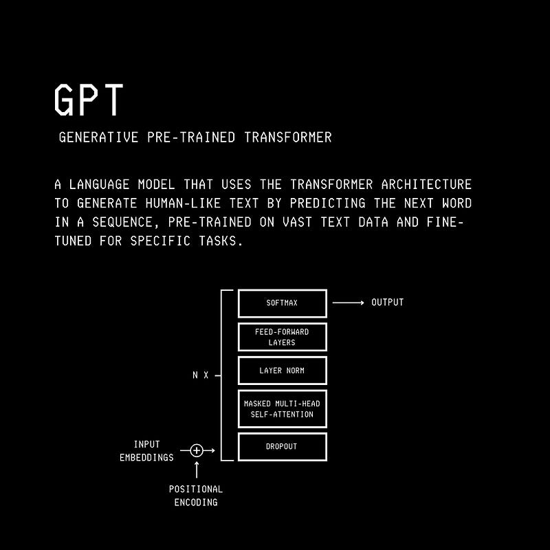
Despite their remarkable performance, this architecture is far from how human cognition works.
Instead of thinking in words, humans understand, reason about and generate ideas at multiple levels of abstraction.
Think about a teacher.
They do not plan every spoken word during their lecture.
Instead, in their mind, they outline a flow of high-level ideas they want to discuss.
These ideas can be distinct or depend on each other. They can also be in different languages or modalities (sound, image, text, etc.).
In each case, the teacher never considers every single word associated with them.
Instead, these high-level abstract ideas are translated by adding details at the lower levels of abstraction using different words each time they are discussed.
Such hierarchical high-level abstraction is not explicitly present in the current LLM architecture. (Although they might implicitly learn such representations during their training.)
Building on this insight, Meta researchers published a new architecture called the Large Concept Model or LCM.
Instead of reasoning and processing at the token level, LCMs do these in an abstract embedding space.
This embedding space is designed to be independent of language or modality.
Compare this to the current LLMs that are English-centric and token-based.
LCMs process, reason in and generate abstract atomic ideas called ‘Concepts’ that could correspond to a sentence in a text document or an equivalent speech utterance in an audio clip. (These could even be smaller or larger than a sentence/ single utterance.)
These generated Concepts can be decoded into any language and modality (that is supported by the embedding) in a purely zero-shot fashion without re-training the model.
Interestingly, they outperform existing LLMs of similar size in this task and compare well with them in other language-based tasks.
Here is a story where we deep dive into how Large Concept Models work and see how they stand next to state-of-the-art LLMs.
Let’s begin!
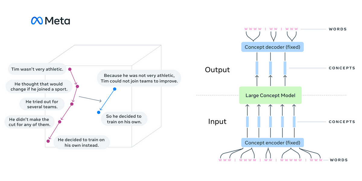
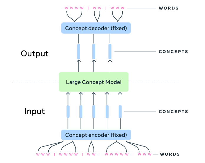
An Overview Of How An LCM Works
A Large Concept Model or LCM takes an input of ‘Concepts’.
For a text dataset, it is first segmented into sentences of 10 to 20 tokens in length. These sentences represent ‘Concepts’ for the model.
(Note that a ‘Concept’ can even be bigger than a sentence.)
These sentences are converted into embeddings using SONAR. (We will come back to this soon.)
The sequence of sentence embeddings is then fed to the LCM, which processes them to output a new sequence of embeddings.
These embeddings are again decoded back to sentences (Concepts) using SONAR.
The encoder and decoder used in the process are fixed and not trained with the model.
It is interesting to note that the output of an LCM can be decoded into any other language or modality, irrespective of the input language or modality, without performing any repeat processing.
Let’s understand this process step by step.
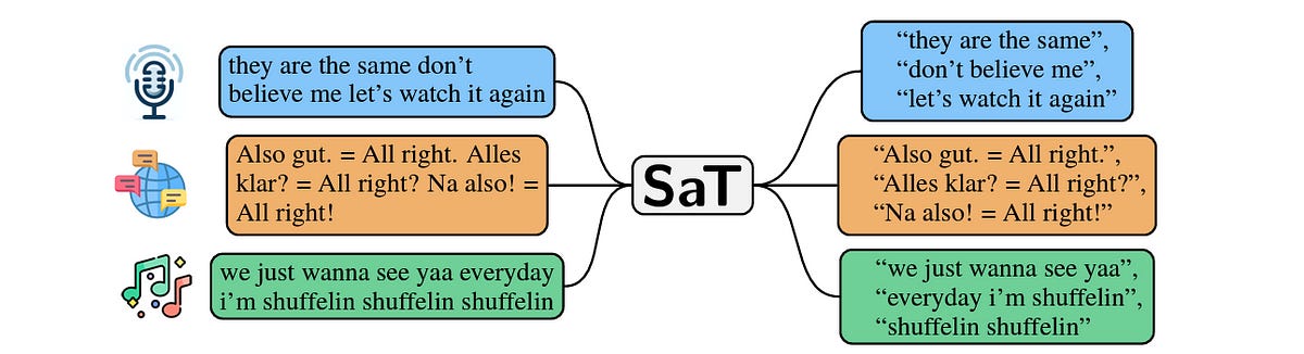
How Is Text Broken Down Into Sentences?
The process starts with segmenting large corpora of text into sentences.
Reserachers use the Segment any Text (SaT) technique for this.
Segmentation is capped at 200 characters, as they found that this number produces the best results in their evaluations.
How Are The Concept Embeddings Generated?
Sentences are then converted into embeddings using SONAR or Sentence-Level Multimodal and Language-Agnostic Representations.
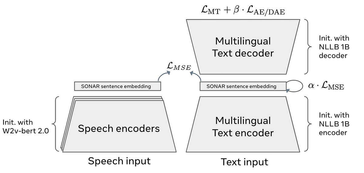
SONAR embeddings are trained as an NLLB-1B Encoder/ Decoder architecture using the Mean Square Error (MSE) loss.
After training the text embeddings, they are extended to the speech modality (initialised using the W2v-Bert 2.0 Encoder) using the teacher-student approach of Knowledge Distillation, again using the MSE loss.
SONAR impressively supports 200 languages for text processing into and out of English and 76 languages for speech input and output in English.
The LCM Architecture
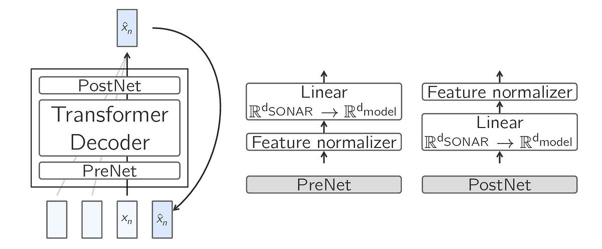
The Large Concept Model is essentially a decoder-only Transformer that is enhanced using two additional components that handle Concept embeddings.
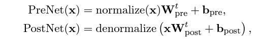
These are called Pre-Net and Post-Net.
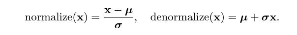
The PreNet normalizes the SONAR embeddings and maps them into the model’s hidden dimension.
The PostNet reverses the normalization and maps the model’s outputs back into the SONAR embedding space.
The researchers termed this structure the Base-LCM (as there are a few more LCM variants).
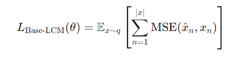
The LCM operates with the next-concept (next-sentence embeddings) prediction objective.
In other words, it predicts the next Concept based on the preceding ones (in an autoregressive manner).
This is done by minimizing the Mean Squared Error (MSE) between the predicted and the ground truth embedding.
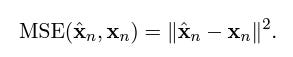
For a data distribution of sequences of concepts denoted by q, the overall training loss is shown below:
An ‘End of Text’ (eot) suffix is added to the end of the sequence of concepts, and this suffix is encoded using SONAR as well.
The model learns to predict this token to indicate the end of the sequence.
At inference time, text generation stops based on two conditions:
The cosine similarity between the generated embedding and the
eotembedding crosses a certain threshold (represented bys(eot))The cosine similarity between consecutive embeddings crosses a certain threshold (represented by
s(prev))
Both s(eot) and s(prev) are set to 0.9 in the original model implementation.
Moving Forward To A Diffusion Based LCM
Training the Base-LCM by minimizing MSE loss results in the model producing deterministic responses and predicting an average representation of all possible continuations.
This averaged embedding might not have any meaningful translation.
It might also not be creative enough for language tasks with multiple valid continuations.
To fix the poor results obtained by the Base LCM, researchers use Diffusion with the model so that it can generate meaningful and diverse next-concept embeddings, probabilistically.
With Diffusion, an LCM can learn a conditional probability distribution over sentence embeddings and sample from it during inference time.
Similar to how diffusion generates images, in a Diffusion-based LCM, a forward noising process adds noise to sentence embeddings, and a reverse denoising process is used to predict the original noiseless embeddings.
Let’s learn this in more detail.
The Two Steps Of Diffusion
In the Forward noising process, sentence embeddings (x(0)) are gradually corrupted (noised) with Gaussian noise over a series of timesteps (t) to produce noisy embeddings (x(t)).
A Noise schedule determines how the added noise increases over time.
This process is shown using the equation below:

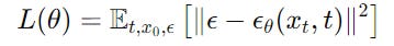
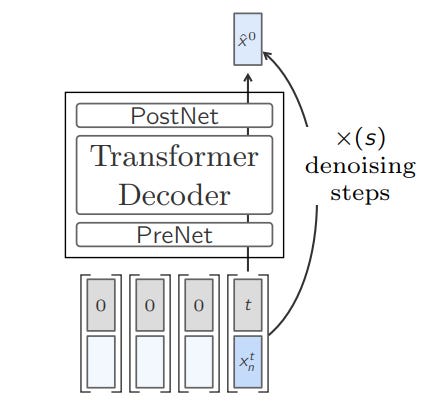
In the Reverse denoising process, a Transformer-based model is trained to predict the original or noiseless embeddings (x(0)) from the noisy embeddings (x(t)).

The objective for training a Diffusion model is to minimize the reconstruction error of the clean embeddings.
During inference time, the model starts with pure Gaussian noise and iteratively denoises it to produce embeddings.
There’s another idea that is important to learn before we discuss Diffusion-based LCMs. This is Classifier-Free Guidance.
Classifier-Free Guidance (CFG)
This is a technique that allows diffusion models to generate outputs based on a given conditioning input without requiring a separate classifier.
For example, generating an image based on a prompt.
(Before the invention of CFG, a separate classifier was trained with a diffusion model that guided the generation process aligned to a conditioning input. This technique was called Classifier-based guidance.)
Classifier-free guidance works by training a diffusion model to generate both conditioned (output p(x ∣ y), where y is the conditioning variable) and unconditioned outputs (output p(x)).
At inference time, the model combines these to balance generation quality and diversity using the following equation:

Influenced by the processes described above, two LCM variants are created:
One-Tower Diffusion LCM
Two-Tower Diffusion LCM
Let’s discuss them further.
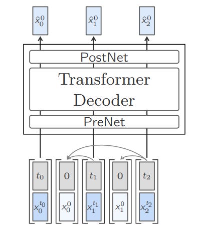
One-Tower Diffusion LCM
This LCM uses a single Transformer for both noising and denoising processes.
Since just one component is involved in processing, the model is called ‘One-Tower’.
It predicts the clean next sentence embedding given a noisy input conditioned on previous embeddings.
First, each embedding is concatenated with the corresponding diffusion timestep embedding to give the model information about the noise level.
Next, learned position embeddings are added to the input embeddings to encode the sequential structure.
This prepares the embeddings that are fed to the LCM.
The Transformer of the LCM uses Causal multi-head self-attention to process this sequence of embeddings.
During training, the input consists of interleaved noisy and clean embeddings, and the attention mask is specifically designed to allow the noisy embeddings to attend only to the clean embeddings.
This teaches the model to condition its denoising process properly.
To enable classifier-free guidance at inference time, Self-attention is occasionally dropped based on a certain probability during training.
This allows the model to learn both conditional and unconditional generation.
Two-Tower Diffusion LCM
This architecture consists of two components or ‘Towers’ that handle processing context and denoising separately.
The first Tower is called Contextualizer.
This is a decoder-only Transformer with Causal Self-attention which is tasked to encode the preceding context embeddings.
The outputs of this tower are fed to the second tower called the Denoiser.
This tower consists of a stack of Transformer blocks with Cross-attention, which is tasked to iteratively denoise the noisy next embedding to predict the clean embedding.
Each layer of the denoiser uses the Adaptive Layer Normalization (AdaLN) mechanism that helps modulate it to handle varying levels of noise during the denoising process.
Also, the Self-attention layers in the denoiser only attend to the current position and not the preceding noised context.
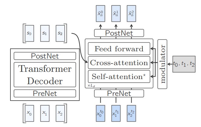
During training, rows of the Cross-attention mask in the denoiser are randomly dropped with a certain probability. This enables classifier-free guidance during inference.
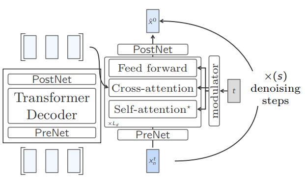
At inference time, the model starts with a random noise vector.
The denoiser iteratively denoises it guided by the context from the contextualizer and the AdaLN-modulated cross-attention.
There’s A Quantized LCM As Well
Lastly, another variant of LCM is trained where, instead of using the continuous sentence embeddings from the SONAR space, these are quantized or converted into a discrete form.
A technique called Residual Vector Quantization (RVQ) is used for this process.
Two models, Quant-LCM-d and Quant-LCM-c, are then trained.
The former predicts discrete units, while the latter predicts continuous residuals to refine embeddings during the generation process.
Which LCM Variants Perform The Best?
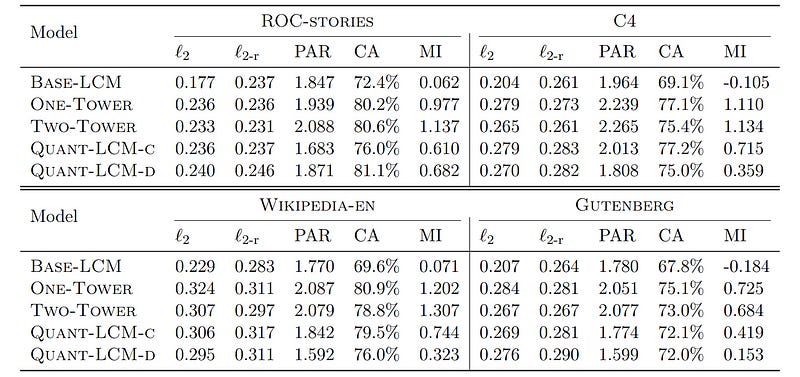
All four LCM variants with 1.6 billion trainable parameters are first pre-trained on the Fineweb-edu dataset.
Performance on Pre-Training
When Pre-training is evaluated, Base-LCM shows the lowest L2 scores but the poorest performance on Contrastive accuracy (CA) and Mutual information (MI) compared to Diffusion-based LCMs and Quant-LCM.
The reason?
Since many valid next-sentence continuations exist for a given context when Base-LCM generates an average next-sentence continuation (by optimizing MSE loss), this may not correspond to any meaningful embedding in the SONAR space.
Also, if you’re new to these metrics —
Contrastive Accuracy (CA) measures whether the predicted embedding is closer to the true next-sentence embedding than to other unrelated embeddings in the batch.
Mutual Information (MI) measures how well the predicted sentence aligns contextually with the preceding sentences.
Both Diffusion-based models attain the highest mutual information (MI) with no consistent performance difference between them.
This shows that the embeddings they produced effectively align with realistic text continuations.
Performance on Instruction-tuning
All pre-trained models are next fine-tuned on the Cosmopedia dataset.
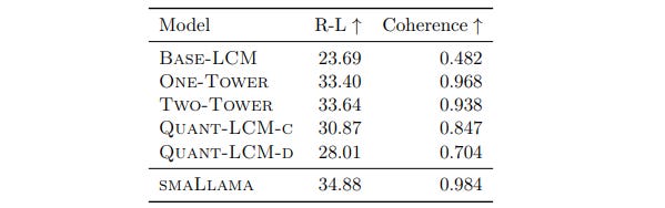
Upon evaluation, Diffusion-based models outperform both Quant-LCM and Base-LCM.
A small Llama model with 24 transformer layers and 1.4 billion parameters is pre-trained and fine-tuned in similar ways and compared to the LCMs as well.
Notably, this model, called SmaLlama, still outperforms all LCM models on the given metrics, pointing towards better fluency of generated text.
How Do LCMs Compare With LLMs?
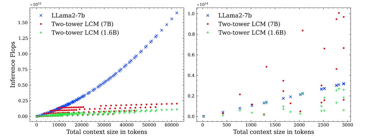
Inference Efficiency
LCMs work with Concepts rather than tokens, which leads to shorter embeddings.
Since the Attention mechanism used in Transformers has quadratic complexity for the sequence length, the computational cost and interference time for LCMs are far lower than for LLMs.
It is only for extremely short sentences (<10 tokens) that an LLM is more computationally efficient than an LCM.
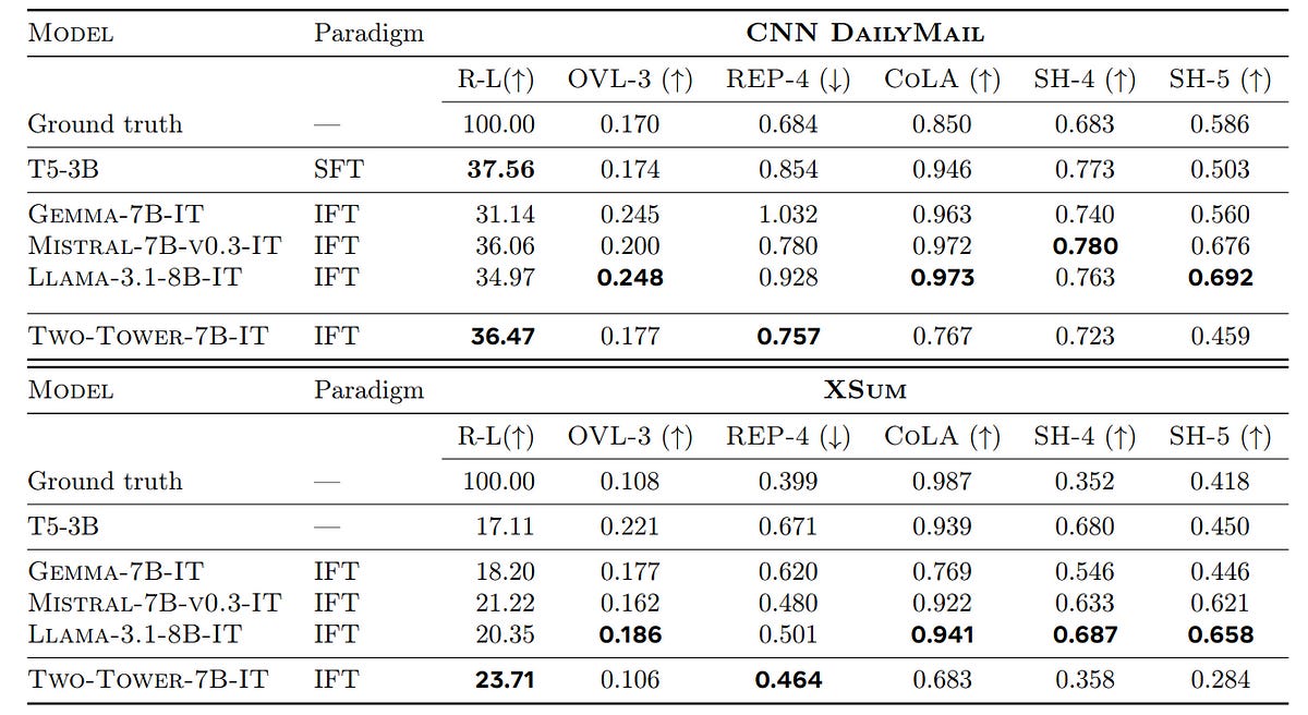
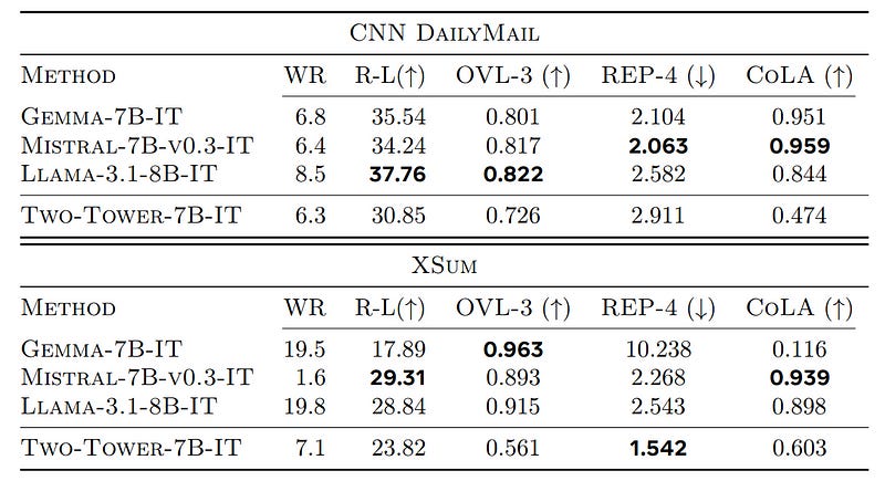
Short-Context Summarization Task
For this task, the Two-Tower LCM scaled to 7 billion parameters has competitive generative performance to many instruction fine-tuned LLMs (higher ROUGE-L score), has fewer repetitions in the generated text (lower REP-4 score) and generates more abstractive summaries (lower OVL-3 score).
On the other hand, it is less fluent than other LLMs (lower CoLA score).
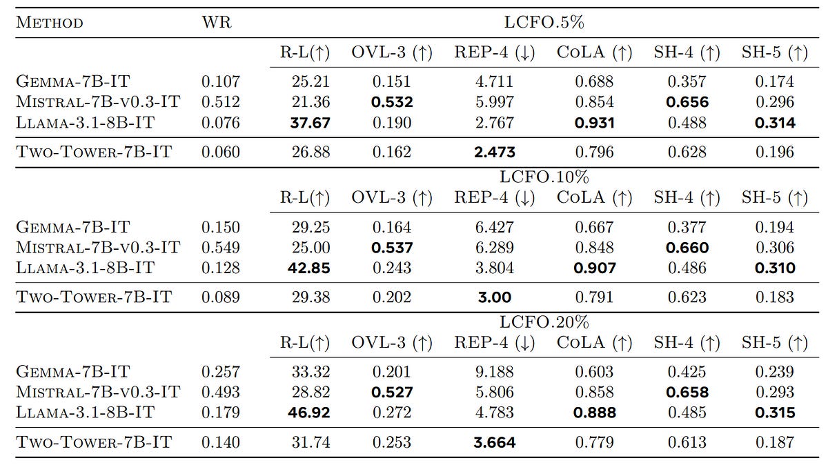
Long-Context Summarization Task
When evaluated for this type of task on the LCFO dataset, the Two-Tower LCM outperforms Mistral-7B-v0.3-IT and Gemma-7B-IT (higher ROUGE-L score) for compressed summary tasks (5% and 10% of source length).
LCM also has high semantic relevance for the summaries to the source for all conditions (high SH-5 score).
Summary Expansion Task
On this task of generating longer text for a given summary, LLMs get higher ROUGE-L scores than LCMs.
LCMs generate more paraphrased content but score lower on fluency.
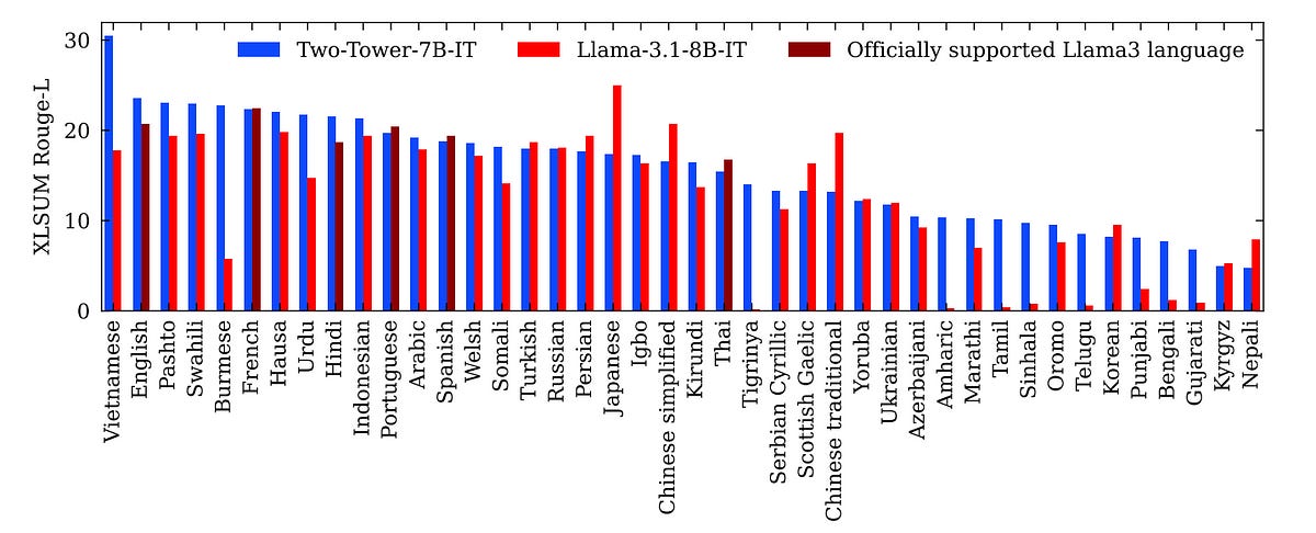
Zero-Shot Multi-Lingual Performance
SONAR embeddings support text in 200 languages and speech in 76 languages.
When an LCM, backed by SONAR, is evaluated on the XL-Sum dataset for multilingual abstractive summarization in 42 languages, its results are quite impressive.
As compared to Llama-3.1–8B-IT (that has been fine-tuned in different languages), Two-Tower LCM (that has never seen training data language other than English) scores higher in Multilingual ROUGE-L score in English and other languages supported by both models.
LCMs also generalize well to other low-resource languages (like Vietnamese, Hausa and Burmese) in a zero-shot setting (languages it has never seen before).
LLMs Still Remain Undefeated. But For How Long?
LLMs stand strong in these evaluations.
This is because next-sentence (Concept) prediction is more challenging than next-token prediction.
This is because the number of possible sentences, given some context, is virtually unlimited. (Compare this to token vocabularies that are usually in the range of 100k.)
LLMs produce logits for each token in the vocabulary and then use a Softmax output to convert these into probabilities.
The token with the highest probability is selected as the next token (if using Greedy decoding), or it can be sampled based on a probability distribution (Temperature sampling).
LCMs, on the other hand, generate text in a continuous embedding space rather than choosing tokens from a vocabulary.
Such a probability distribution can theoretically be learned using Diffusion (and that’s why Diffusion-based LCMs perform better than others), but they are still not at their best.
LCMs still have a long way to go to reach the performance of current state-of-the-art LLMs, but they are really promising contenders.
It would be exciting to see how their story unfolds when blindly scaling LLMs no longer works.
Further Reading