ML Interview Essentials: What Is Normalization?

#2: A deep dive into how Normalization works, and why it is so effective. (6 minutes read)

Dr. Ashish Bamania

Nov 09, 2025

Comparison between different normalization methods. C represents the number of Channels/ embedding dimension, N is the Batch size (called B in text), and H x W represents the number of tokens (T = H × W) (Source: ArXiv research paper titled ‘Group Normalization’)

Normalization is an indispensable part of today's AI models, but this topic doesn’t get as much attention as it should.

We are going to fix this today with this article.

This is the second article in the series designed to help you succeed in ML interviews.

Read the previous article on Self-attention, if you missed it earlier, using the link below:

ML Interview Essentials: Building Self-Attention From Scratch

Dr. Ashish Bamania

Nov 2

Read full story

What Is Normalization?

Neural networks are notoriously hard to train.

During training, the distribution of inputs to each layer in a neural network can shift as the parameters in earlier layers change. This is called Internal covariate shift.

To fix this unwanted distribution shift, a technique called Normalization is used, which adjusts and scales the outputs (activations) of neurons in the neural network.

Take an input tensor x with shape (B,T,C) where:

B is the batch size/ number of samples
T is the number of tokens in a sample
C is the embedding dimension

For example, a batch of 32 sentences (B), each tokenized into 128 tokens (T), and each token represented as a 768-dimensional vector (C), has a shape of (32, 128, 768).

Normalization is applied to this tensor using the formula:

where:

γ and β are learnable parameters of shape (C, ) for scaling and shifting the output (affine transformation)
ϵ is a small constant added to the denominator to prevent division by zero (without it, it could lead to exploding gradients)
μ and σ² are the mean and variance of the input tensor. These are computed differently based on the method being used, as discussed next.

It was in 2015 when researchers at Google published a research paper on Batch Normalization.

Batch Normalization (BatchNorm or simply BN), which was primarily intended to be used in CNNs, involves computing the mean μ and variance σ² for each channel C indexed by k across both the batch (B) and token dimensions (T) as:

Mean in the Batch Normalization formula is computed for each channel, indexed by k, across the batch and token dimensions, indexed by i and j, respectively.

Variance in the Batch Normalization formula is computed for each channel, indexed by k, by averaging the squared deviations from the mean across the batch and token dimensions, indexed by i and j, respectively.

(Note that we use the term “Channel” to refer to C when we talk about CNNs/ Vision models. It is also called “Feature dimension” in a general machine learning context and “Embedding dimension” in the context of language or sequence models.)

BatchNorm was soon applied to a variety of vision models and became widely successful (the paper received the ICML Test Of Time Award 2025).

Following it came many other types of normalization layers, namely:

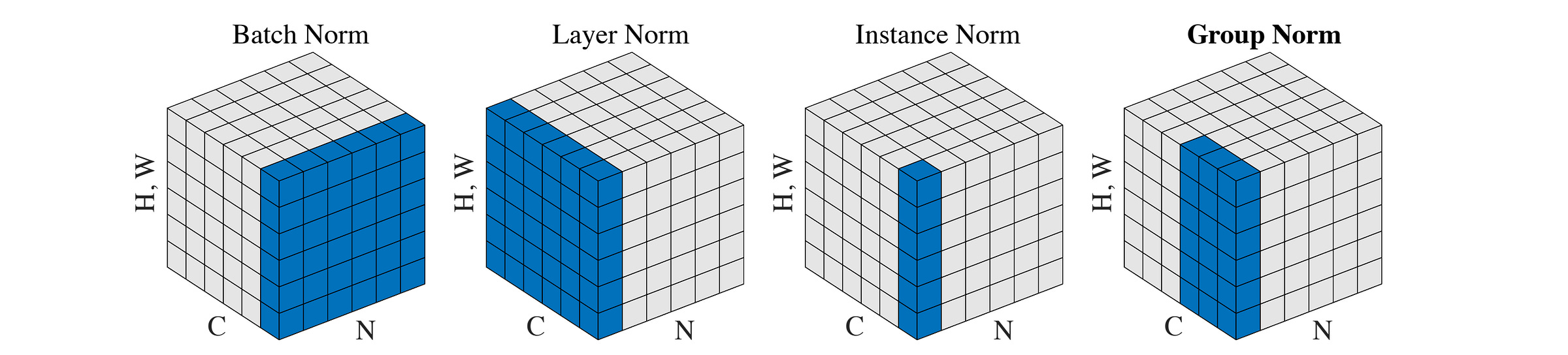
As we previously discussed, the differences between them lie in how the mean and variance are calculated over the input.

While BatchNorm calculates them across the batch (B) and token (T) dimensions for each channel (C), they are calculated in:

InstanceNorm: across tokens (T), for each sample (B) and each channel (C)
GroupNorm: across groups of channels (C) and tokens (T), for each sample (B)
LayerNorm: across all channels (C), for each sample (B) and each token (T)

In the context of CNNs, LayerNorm computes these statistics across both channels (C) and spatial dimensions (H x W), for each sample (represented by B or N in the image), as shown below.

While GroupNorm and InstanceNorm are used to improve object detection and image stylization, LayerNorm (and its variant RMSNorm) has become the de facto layer in Transformer-based architectures.

In LayerNorm, the mean (per sample and token) is calculated as:

Mean in the Layer Normalization formula is computed across all channels C, indexed by k, independently for each sample i (out of a total of B) and each token j (out of a total of T).

And the variance is calculated as:

Variance in the Layer Normalization formula is computed across all channels C, indexed by k, independently for each sample i (out of a total of B) and each token j (out of a total of T).

The general normalization formula that we previously discussed:

becomes the following for LayerNorm (LN):

Layer normalization visualised (Image from author’s book “LLMs In 100 Images”)

Building on this, a 2019 research paper introduced Root Mean Square Layer Normalization (RMSNorm), a computationally simpler and thus more efficient alternative to LayerNorm.

It removes the step of subtracting the mean from the input tensor (Mean centering) and normalizes the input using the RMS or Root Mean Square value as below:

This makes the RMSNorm formula (note the emission of the affine shift β term):

RMSNorm is used today in LLaMA, Mistral, Qwen, DeepSeek, and OpenELM series of LLMs. GPT-2 on the other hand, uses LayerNorm.

It is seen that normalization layers help optimize training and enable neural networks to achieve faster convergence with better generalization.

But what do Normalization layers do internally that leads to such impressive results?

What Makes Normalization Work So Well

To answer this question, we look into a Meta research paper where the authors use three different Transformer models, namely:

a Vision Transformer model (ViT-B) trained on the ImageNet-1K dataset
a wav2vec 2.0 Large Transformer model trained on the Librispeech audio dataset
a Diffusion Transformer (DiT-XL) trained on the ImageNet-1K dataset

All of the above models have LayerNorm applied in every Transformer block and before the final linear projection.

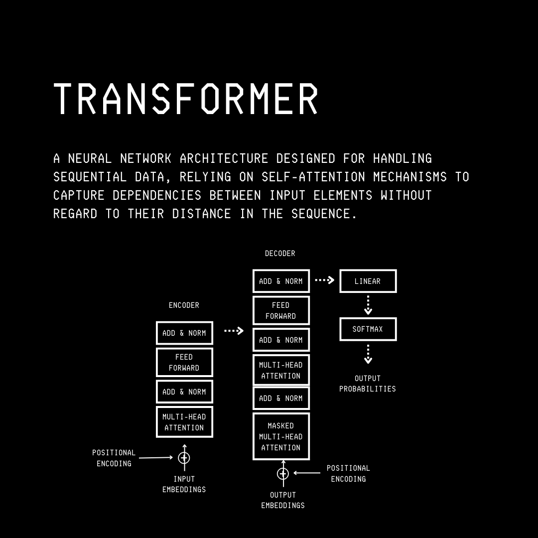
The following visualisation shows the Transformer architecture as a refresher.

Transformer visualised (Image from author’s book “LLMs In 100 Images”)

A mini-batch of samples is used during the forward pass through these models.

Next, the tensor inputs and outputs (measured before the scaling and shifting operations) from normalization layers at varying depths in the network are measured and plotted to examine how normalization layers affect them.

The following is how these plots look.

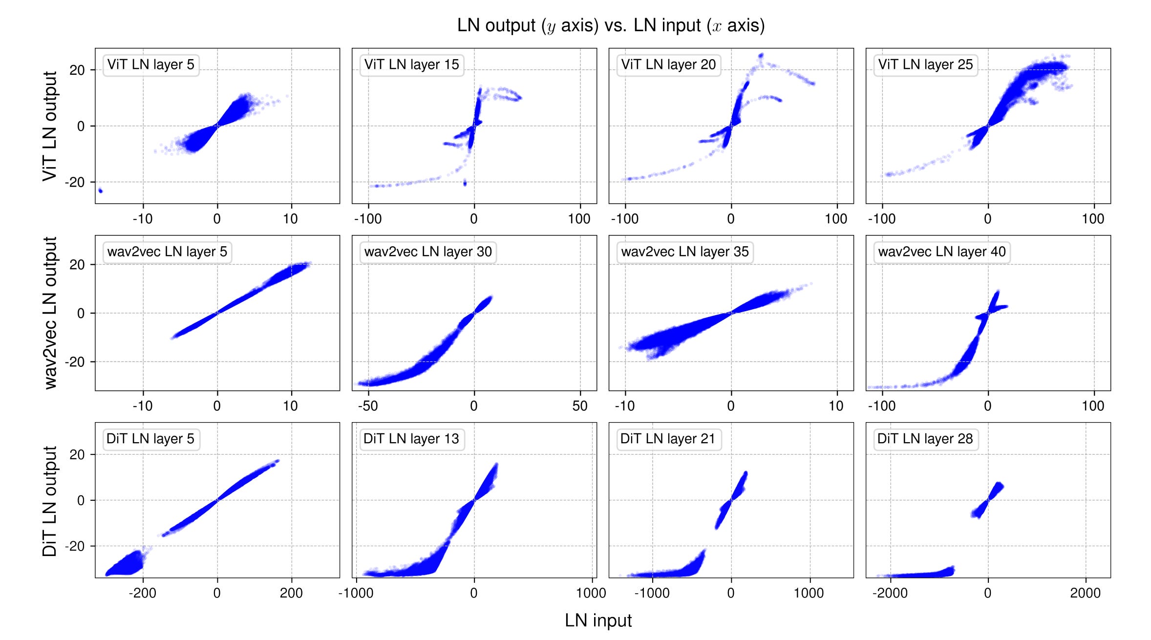
Output (on y-axis) vs. input (on x-axis) of four different LayerNorm layers at different depths in ViT, wav2vec 2.0, and DiT models. Plots on the left-sided columns are for the earlier layers.

It is clear that there is a linear input-output relationship (seen as a straight line in the plot) in the earlier LayerNorm layers of all three models.

But something interesting happens as we move towards deeper LayerNorm layers.

It is seen that these plots are no longer a straight line, but rather resemble an S-shaped curve, similar to a hyperbolic tangent (tanh) function.

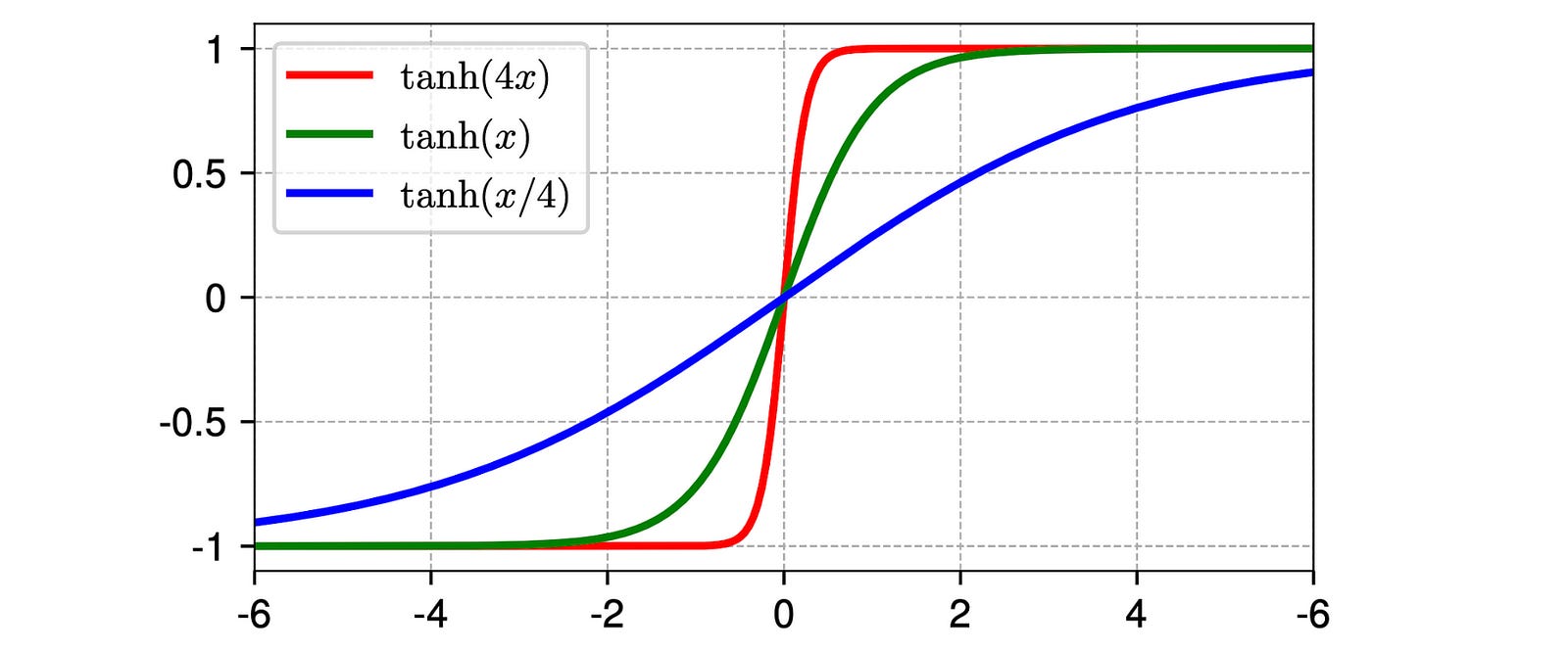
Plots of the tanh(αx) function with three different α values

This is quite strange.

One would expect that LayerNorm would linearly transform the input tensor since its constituent operations (subtracting the mean and dividing by the standard deviation) are linear.

Why do we see an S-shaped curve then?

This is because LayerNorm normalizes in a per-token manner. It linearly transforms each token’s activations.

Since different tokens in an input tensor can have different mean and standard deviation values, when the results are plotted collectively, the total input tensor is seen not to be transformed linearly.

Note how LayerNorm brings the extreme values of token activations (for example, input values larger than 50 or smaller than -50 in the plots) in line with the majority of points. This leads to the non-linear ends of the S-shaped curve.

On the other hand, smaller values (closer to zero) still contribute to the linear shape in the central part of the S-shaped curve.

This disproportionate squashing effect of LayerNorm on extreme values aligns with how biological neurons function, which is a reason why normalization layers achieve better results in neural network training.

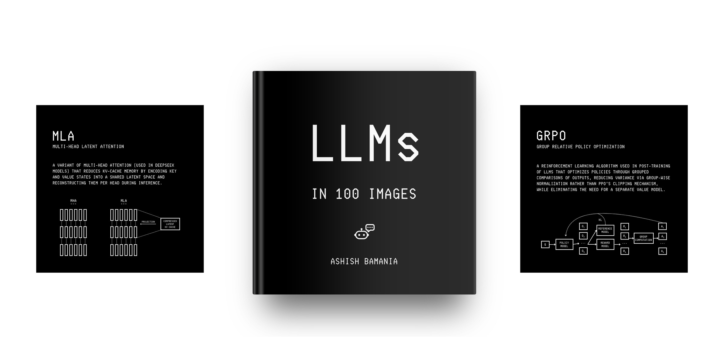
Images used in this article are taken from my book ‘LLMs In 100 Images’.

It is a collection of 100 easy-to-follow visuals that explain the most important concepts you need to master to understand LLMs today.

Grab your copy today at a special early bird discount using this link.