ML Interview Essentials: What Is Gradient Descent

#3: Gradient Descent (6 minutes read)

Nov 13, 2025

👋🏻 Hey there!

This article is a part of the ML interview essentials series on the publication.

If you have not read the previous articles in this series, here is your chance to get interview-ready like never before.

ML Interview Essentials: Building Self-Attention From Scratch

Dr. Ashish Bamania

Nov 2

Read full story

ML Interview Essentials: What Is Normalization?

Dr. Ashish Bamania

Nov 9

Read full story

Let’s begin!

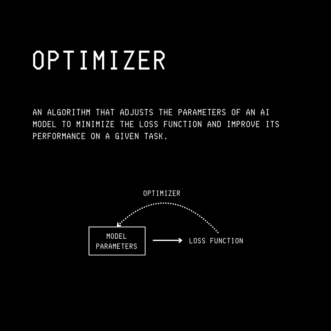
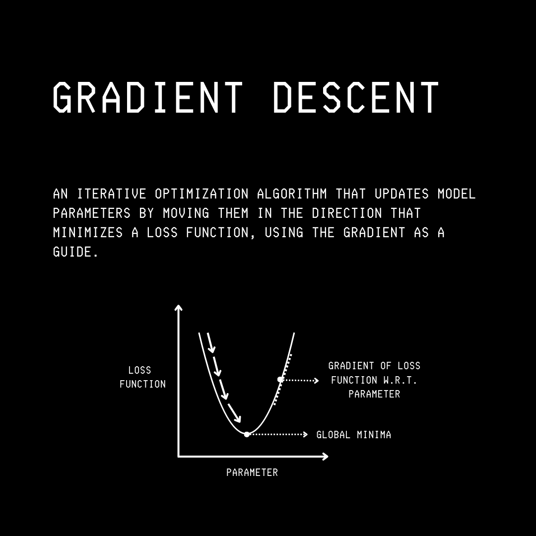
Gradient Descent (also called Batch Gradient Descent or BGD) is an iterative optimization algorithm (optimizer).

It minimizes a loss function by moving the model parameters (weights and biases) in the direction of the steepest descent towards the global minimum.

This helps us find the model parameters that achieve the best accuracy.

Optimizer visualised (Image from author’s book titled ‘**AI In 100 Images**’)

Mathematically, given J(θ), a loss function with respect to model parameters θ, gradient descent updates model parameters as follows:

where:

θ(t+1) is the value of the updated parameters after applying one gradient descent iteration
θ(t) is the value of the parameters at iteration (or timestep) t
η is the learning rate, a small positive scalar that controls the step size of gradient descent
∇J(θ(t)) is the gradient of the loss function J with respect to the parameters θ,
evaluated at the current parameters θ(t)

Gradient descent visualised (Image from author’s book titled ‘**LLMs In 100 Images**’)

The Mathematics Of Gradient Descent

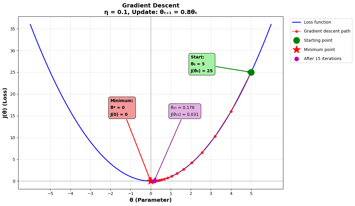
Let’s use a simple loss function that represents a parabola with a minimum at θ = 0.

The gradient of this function is:

Let’s use a learning rate of η = 0.1 and derive the gradient descent update equation:

This means that at each iteration or timestep, we need to multiply the model parameters by 0.8 till the model converges to the lowest value of the loss function.

In other words, with gradient descent, the parameter converges to the minimum, decreasing by 20% at each step.

Let’s say that the initial value of the parameter θ represented by θ(0) was 5.

Over the iterations, the parameter values will be as follows:

Iteration 0: θ₀ = 5
Iteration 1: θ₁ = 0.8 × 5 = 4.0
Iteration 2: θ₂ = 0.8 × 4.0 = 3.2
Iteration 3: θ₃ = 0.8 × 3.2 = 2.56
Iteration 4: θ₄ = 0.8 × 2.56 = 2.048
Iteration 5: θ₅ = 0.8 × 2.048 = 1.638
Iteration 15: θ₁₅ ≈ 0.176
Iteration 30: θ₃₀ ≈ 0.0062

But what’s the minimum value of the loss function, you’d ask. Let’s find out.

The maximum or minimum of a function occurs where its derivative equals zero. Such a point is called the Critical point.

For our loss function, the derivative is:

To find the critical point, we set the derivative equal to zero and solve for θ:

We find that the critical point occurs at θ = 0.

Next, we calculate another derivative of the first derivative equation to determine whether this critical point is a maximum or minimum (Second derivative test):

According to the second derivative test:

If J’‘(θ) < 0, the critical point is a local maximum (the function is concave down).
If J’‘(θ) > 0, the critical point is a local minimum (the function is concave up).

Since J’‘(0) = 2, which is greater than 0 in our case, the critical point at θ = 0 is a local minimum.

This means that the loss function achieves its minimum value at θ = 0, and that minimum value is J(0) = 0.

Building Gradient Descent In PyTorch

Let’s learn to code Gradient descent in Python.

We will use PyTorch in this example, which is one of the most popular libraries for building ML models.

If you’re new to PyTorch, please consider getting familiar with it using the following article.

20 PyTorch Concepts, Explained Simply

Dr. Ashish Bamania

Nov 7

Read full story

import torch

# Create parameter θ
theta = torch.tensor(5.0, requires_grad=True) # Enable gradient tracking

# Define hyperparameters
eta = 0.1 # Learning rate
total_steps = 15 # No. of iterations

print(”Step 0 (initial θ):”, theta.item())
print(”Initial loss:”, (theta ** 2).item())
print()

# Iterate for total_steps 
for step in range(1, total_steps + 1):
    # Forward pass
    loss = theta ** 2
    
    # Backward pass (calculates d(θ²)/dθ = 2θ and stores in theta.grad)
    loss.backward() 
    
    # Store gradient and loss to print later
    gradient = theta.grad.item()
    loss_value = loss.item()

    # Gradient descent update: θ = θ - η·∇J(θ)
    # Use no_grad() to prevent PyTorch from tracking this parameter update
    with torch.no_grad():
        theta -= eta * theta.grad

    print(f”Step {step}:”)
    print(f”loss = {round(loss_value, 3)}”)
    print(f”θ = {round(theta.item(), 3)}”)
    print(f”gradient = {round(gradient, 3)}”)
    print(f”update = {round(eta * gradient, 3)}”)
    print()

    # Reset gradients for next iteration
    theta.grad.zero_()

print(”Final θ:”, round(theta.item(), 3))
print(”Final loss:”, round((theta ** 2).item(), 3))

Here is the output that we obtain.

Step 0 (initial θ): 5.0
Initial loss: 25.0

Step 1:
loss = 25.0
θ = 4.0
gradient = 10.0
update = 1.0

Step 2:
loss = 16.0
θ = 3.2
gradient = 8.0
update = 0.8

Step 3:
loss = 10.24
θ = 2.56
gradient = 6.4
update = 0.64

Step 4:
loss = 6.554
θ = 2.048
gradient = 5.12
update = 0.512

Step 5:
loss = 4.194
θ = 1.638
gradient = 4.096
update = 0.41

Step 6:
loss = 2.684
θ = 1.311
gradient = 3.277
update = 0.328

Step 7:
loss = 1.718
θ = 1.049
gradient = 2.621
update = 0.262

Step 8:
loss = 1.1
θ = 0.839
gradient = 2.097
update = 0.21

Step 9:
loss = 0.704
θ = 0.671
gradient = 1.678
update = 0.168

Step 10:
loss = 0.45
θ = 0.537
gradient = 1.342
update = 0.134

Step 11:
loss = 0.288
θ = 0.429
gradient = 1.074
update = 0.107

Step 12:
loss = 0.184
θ = 0.344
gradient = 0.859
update = 0.086

Step 13:
loss = 0.118
θ = 0.275
gradient = 0.687
update = 0.069

Step 14:
loss = 0.076
θ = 0.22
gradient = 0.55
update = 0.055

Step 15:
loss = 0.048
θ = 0.176
gradient = 0.44
update = 0.044

Final θ: 0.176
Final loss: 0.031

The iterations of gradient descent till step 15 are shown in the plot below.

Variants of Gradient Descent

Gradient descent is the foundational optimization algorithm used in machine learning and deep learning.

But it is not used in its original form, due to some problems associated with it:

It requires computing the gradient over the entire dataset before every update. This can be extremely slow for large datasets.
It uses a fixed learning rate, which may lead to optimization overshooting or moving too slowly towards the minima.
It is sensitive to scale, which means that if gradients differ in size across parameters, convergence can become uneven or unstable.
It can get stuck in local minima, plateaus, or saddle points rather than reaching the global minimum.

To address these issues, two variants of gradient descent are popularly used.

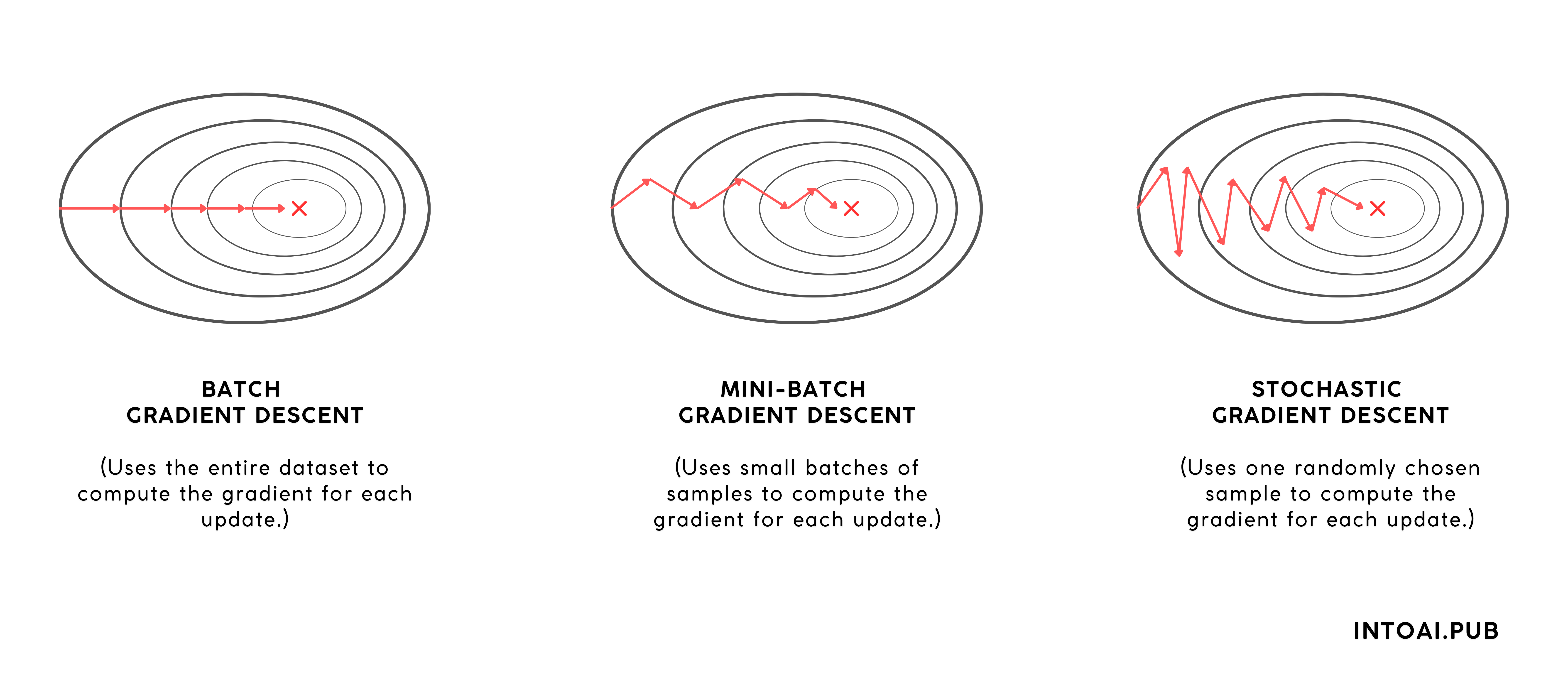
1. Stochastic Gradient Descent (SGD)

SGD uses one random sample from the dataset at a time to compute gradients.

This leads to rapid updates and helps SGD escape local minima due to its noise.

However, sometimes the noisy convergence (high variance in updates) may prevent it from converging to the global minimum.

In comparison, Batch Gradient Descent (BGD) converges more stably and provides more deterministic updates.

2. Mini-Batch Gradient Descent

Mini-batch Gradient Descent uses small batches (e.g., 32, 64, 256 samples from the dataset) at a time to compute gradients.

This achieves the best trade-off between the speed of SGD and the stability of BGD, making it more widely used than either.

Apart from these variants, there are many more advanced optimization algorithms that use:

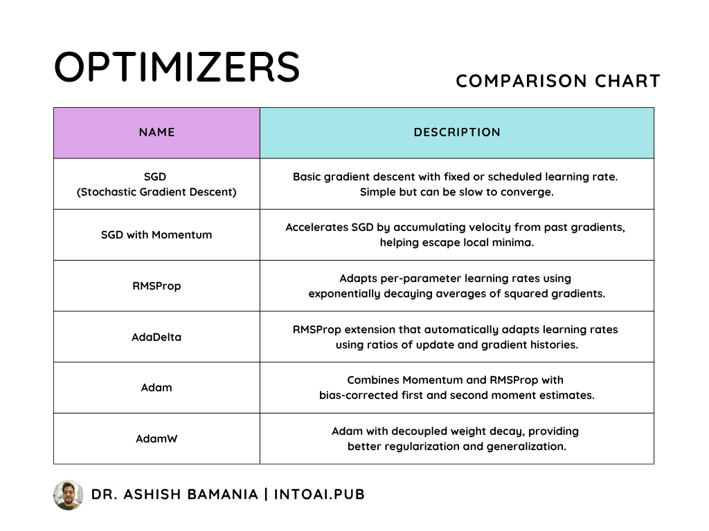
Momentum: Adds a fraction of the previous update direction (called velocity) to the current gradient, allowing the optimizer to build up speed in consistent directions and avoid rapid oscillations. (For example, SGD with momentum)
Adaptive learning rates for each parameter (For example, AdaGrad, RMSProp, and AdaDelta)
A combination of both of these (For example, Adam, AdaMax, and AdamW)